Quadratic Arithmetic Programs

A quadratic arithmetic program is an arithmetic circuit, specifically a Rank 1 Constraint System (R1CS) represented as a set of polynomials. It is derived using Lagrange interpolation on a Rank 1 Constraint System. Unlike an R1CS, a Quadratic Arithmetic Program (QAP) can be tested for equality in $\mathcal{O}(1)$ time via the Schwartz-Zippel Lemma.

Key ideas

In the chapter on the Schwartz-Zippel Lemma, we saw that we can test if two vectors are equal in $\mathcal{O}(1)$ time by converting them to polynomials, then running the Schwartz-Zippel Lemma test on the polynomials. (To clarify, the test is $\mathcal{O}(1)$ time, converting the vectors to polynomials creates overhead).

Because a Rank 1 Constraint System is entirely composed of vector operations, we aim to test if

$$\mathbf{L}\mathbf{a}\circ\mathbf{R}\mathbf{a}\stackrel{?}{=}\mathbf{O}\mathbf{a}$$

holds in $\mathcal{O}(1)$ time instead of $\mathcal{O}(n)$ time (where $n$ is the number of rows in $\mathbf{L}$, $\mathbf{R}$, and $\mathbf{O}$).

But before we do that, we need to understand some key properties of the relationship between vectors and polynomials that represent them.

For all math here, we assume we are working in a finite field, but we skip the $\mod p$ notation for succinctness.

Homomorphisms between vector addition and polynomial addition

Vector addition is homomorphic to polynomial addition

If we take two vectors, interpolate them with polynomials, then add the polynomials together, we get the same polynomial as if we added the vectors together and then interpolated the sum vector.

Spoken more mathematically, let $\mathcal{L}(\mathbf{v})$ be the polynomial resulting from Lagrange interpolation on the vector $\mathbf{v}$ using $(1, 2, …, n)$ as the $x$ values, where $n$ is the length of $\mathbf{v}$. The following is true:

$$\mathcal{L}(\mathbf{v} + \mathbf{w}) = \mathcal{L}(\mathbf{v}) + \mathcal{L}(\mathbf{w})$$

In other words, the polynomials resulting from interpolating vectors $\mathbf{v}$ and $\mathbf{w}$ are the same as the polynomials resulting from interpolating the vectors $\mathbf{v} + \mathbf{w}$.

Worked example

Let $f_1(x) = x^2$ and $f_2(x) = x^3$ $f_1$ interpolates $(1, 1), (2, 4), (3, 9)$ or the vector $[1,4,9]$ and $f_2$ interpolates $[1,8,27]$.

The sum of the vectors is $[2,12,36]$ and it is clear that $x^3 + x^2$ interpolates that. Let $f_3(x) = f_1(x) + f_2(x) = x^3 + x^2$.

$$ \begin{align*} f_3(1) &= 1 + 1 = 2\\ f_3(2) &= 8 + 4 = 12\\ f_3(3) &= 27 + 9 = 36 \end{align*} $$

Testing the math in Python

Unit testing a proposed mathematical identity doesn’t make it true, but it does illustrate what is happening. The reader is encouraged to try out a few different vectors to see that the identity holds.

import galois
import numpy as np

p = 17
GF = galois.GF(p)

xs = GF(np.array([1,2,3]))

# two arbitrary vectors
v1 =  GF(np.array([4,8,2])) 
v2 =  GF(np.array([1,6,12]))

def L(v):
    return galois.lagrange_poly(xs, v)

assert L(v1 + v2) == L(v1) + L(v2)

Scalar multiplication

Let $\lambda$ be a scalar (specifically, a field element in finite field). Then

$$\mathcal{L}(\lambda \mathbf{v}) = \lambda \mathcal{L}(\mathbf{v})$$

Worked example

Suppose our 3 points are $[3, 6, 11]$. The polynomial that interpolates that is $f(x) = x^2 + 2$. If we multiply the vector by 3 we get $[9, 18, 33]$. The polynomial that interpolates that is

from scipy.interpolate import lagrange

x_values = [1, 2, 3]
y_values = [9, 18, 33]

print(lagrange(x_values, y_values))

#    2
# 3 x + 6

$3x^2 + 6$, which equals $3 \cdot (x^2 + 2)$.

Worked example in code

import galois
import numpy as np

p = 17
GF = galois.GF(p)

xs = GF(np.array([1,2,3]))

# arbitrary vector
v =  GF(np.array([4,8,2]))

# arbitrary constant
lambda_ =  GF(15)

def L(v):
    return galois.lagrange_poly(xs, v)

assert L(lambda_ * v) == lambda_ * L(v)

Scalar multiplication is really vector addition

When we say “multiply a vector by 3” we are really saying “add the vector to itself three times”. Since we are only working in finite fields, we don’t concern ourselves with the interpretation of scalars such as “0.5”

We can think of both vectors under element-wise addition (in a finite field) and polynomials under addition (also in a finite field) as groups.

The most important takeaway from this chapter is

The group of vectors under addition in a finite field is homomorphic to the group of polynomials under addition in a finite field.

This is critical because vector equality testing takes $\mathcal{O}(n)$ time, but polynomial equality testing takes $\mathcal{O}(1)$ time.

Therefore, whereas testing R1CS equality took $\mathcal{O}(n)$ time, we can leverage this homomorphism to test the equality of R1CSs in $\mathcal{O}(1)$ time.

This is what a Quadratic Arithmetic Program is.

A Rank 1 Constraint System in Polynomials

Consider that matrix multiplication between a rectangular matrix and a vector can be written in terms of vector addition and scalar multiplication.

For example, if we have a $3 \times 4$ matrix $A$ and a 4 dimensional vector $v$, then we can write the matrix multiplication as

$$ \mathbf{A} \cdot \mathbf{v} = \begin{bmatrix} a_{11} & a_{12} & a_{13} & a_{14}\\ a_{21} & a_{22} & a_{23} & a_{24}\\ a_{31} & a_{32} & a_{33} & a_{34} \end{bmatrix} \begin{bmatrix} v_1\\ v_2\\ v_3\\ v_4 \end{bmatrix} $$

We typically think of the vector $v$ “flipping” and doing an inner product (generalized dot product) with each of the rows, i.e.

$$ \mathbf{A}\cdot \mathbf{v} = \begin{bmatrix} a_{11}\cdot v_1 + a_{12}\cdot v_2 + a_{13}\cdot v_3 + a_{14}\cdot v_4\\ a_{21}\cdot v_1 + a_{22}\cdot v_2 + a_{23}\cdot v_3 + a_{24}\cdot v_4\\ a_{31}\cdot v_1 + a_{32}\cdot v_2 + a_{33}\cdot v_3 + a_{34}\cdot v_4 \end{bmatrix} $$

However, we could instead think of splitting matrix $A$ into a bunch of vectors as follows:

$$ \mathbf{A} = \begin{bmatrix} a_{11} \\ a_{21} \\ a_{31} \end{bmatrix} , \begin{bmatrix} a_{12} \\ a_{22} \\ a_{32} \end{bmatrix} , \begin{bmatrix} a_{13} \\ a_{23} \\ a_{33} \end{bmatrix} , \begin{bmatrix} a_{14} \\ a_{24} \\ a_{34} \end{bmatrix} $$

and multiplying each vector by a scalar from the vector $\mathbf{v}$:

$$ \mathbf{A}\cdot \mathbf{v} = \begin{bmatrix} a_{11} \\ a_{21} \\ a_{31} \end{bmatrix}\cdot v_1 + \begin{bmatrix} a_{12} \\ a_{22} \\ a_{32} \end{bmatrix}\cdot v_2 + \begin{bmatrix} a_{13} \\ a_{23} \\ a_{33} \end{bmatrix}\cdot v_3 + \begin{bmatrix} a_{14} \\ a_{24} \\ a_{34} \end{bmatrix}\cdot v_4 $$

We have expressed matrix multiplication between $\mathbf{A}$ and $\mathbf{v}$ purely in terms of vector addition and scalar multiplication.

Because we established earlier that the group of vectors under addition in a finite field is homomorphic to the group of polynomials under addition in a finite field, can express the computation above in terms of polynomials that represent the vectors.

Succintly testing that $\mathbf{A}\mathbf{v}_1 = \mathbf{B}\mathbf{v}_2$

Suppose we have matrix $\mathbf{A}$ and $\mathbf{B}$ such that

$$ \begin{align*} \mathbf{A} = \begin{bmatrix} 6 & 3\\ 4 & 7\\ \end{bmatrix}\\ \mathbf{B} = \begin{bmatrix} 3 & 9 \\ 12 & 6\\ \end{bmatrix} \end{align*} $$

and vectors $\mathbf{v}_1$ and $\mathbf{v}_2$

$$ \begin{align*} \mathbf{v}_1 = \begin{bmatrix} 2 \\ 4 \\ \end{bmatrix}\\ \mathbf{v}_2 = \begin{bmatrix} 2 \\ 2 \\ \end{bmatrix} \end{align*} $$

We want to test if

$$ \mathbf{A}\mathbf{v}_1 = \mathbf{B}\mathbf{v}_2 $$

is true.

Obviously we can carry out the matrix arithmetic, but the final check will require $n$ comparisons, where $n$ is the number of rows in $\mathbf{A}$ and $\mathbf{B}$. We want to do it in $\mathcal{O}(1)$ time.

First, we convert the matrix multiplication $\mathbf{A}\mathbf{v}_1$ and $\mathbf{B}\mathbf{v}_2$ to the group of vectors under addition:

$$ \begin{align*} \mathbf{A} &= \begin{bmatrix} 6 \\ 4 \\ \end{bmatrix} , \begin{bmatrix} 3 \\ 7 \\ \end{bmatrix}\\ \mathbf{B} &= \begin{bmatrix} 3 \\ 12 \\ \end{bmatrix} , \begin{bmatrix} 9 \\ 6 \\ \end{bmatrix} \end{align*} $$

We now want to find the homomorphic equivalent of

$$ \begin{bmatrix} 6 \\ 4 \\ \end{bmatrix}\cdot 2+ \begin{bmatrix} 3 \\ 7 \\ \end{bmatrix}\cdot 4\stackrel{?}{=} \begin{bmatrix} 3 \\ 12 \\ \end{bmatrix}\cdot 2= \begin{bmatrix} 9 \\ 6 \\ \end{bmatrix}\cdot 2 $$

in the polynomial group.

Let’s convert each of the vectors to polynomials over the $x$ values $[1,2]$:

$$ \underbrace{ \begin{bmatrix} 6 \\ 4 \\ \end{bmatrix}}_{p_1(x)}\cdot 2+ \underbrace{ \begin{bmatrix} 3 \\ 7 \\ \end{bmatrix}}_{p_2(x)}\cdot 4\stackrel{?}{=} \underbrace{ \begin{bmatrix} 3 \\ 12 \\ \end{bmatrix}}_{q_1(x)}\cdot 2= \underbrace{ \begin{bmatrix} 9 \\ 6 \\ \end{bmatrix}}_{q_2(x)}\cdot 2 $$

We will invoke some Python to compute the Langrage interpolation:

import galois
import numpy as np

p = 17
GF = galois.GF(p)

x_values = GF(np.array([1, 2]))

def L(v):
    return galois.lagrange_poly(x_values, v)

p1 = L(GF(np.array([6, 4])))
p2 = L(GF(np.array([3, 7])))
q1 = L(GF(np.array([3, 12])))
q2 = L(GF(np.array([9, 6])))

print(p1)
# 15x + 8 (mod 17)
print(p2)
# 4x + 16 (mod 17)
print(q1)
# 9x + 11 (mod 17)
print(q2)
# 14x + 12 (mod 17)

Finally, we can check if

$$p_1(x) \cdot 2+ p_2(x) \cdot 4 \stackrel{?}= q_1(x) \cdot 2 + q_2(x) \cdot 2$$

is true by invoking the Schwartz-Zippel Lemma:

import random
u = random.randint(0, p)
tau = GF(u) # a random point

left_hand_side = p1(tau) * GF(2) + p2(tau) * GF(4)
right_hand_side = q1(tau) * GF(2) + q2(tau) * GF(2)

assert left_hand_side == right_hand_side

The final assert statement is able to test if $\mathbf{A}\mathbf{v}_1 = \mathbf{B}\mathbf{v}_2$ doing a single comparison instead of $n$.

R1CS to QAP: Succinctly testing that $\mathbf{L}\mathbf{a}\circ\mathbf{R}\mathbf{a}=\mathbf{O}\mathbf{a}$

Since we know how to test of $\mathbf{A}\mathbf{v}_1 = \mathbf{B}\mathbf{v}_2$ succinctly, can we also test if $\mathbf{L}\mathbf{a}\circ\mathbf{R}\mathbf{a}=\mathbf{O}\mathbf{a}$ succinctly?

The matrices have $m$ columns, so let’s break each of the matrices into $m$ column vectors and interpolate them on $(1, 2, …, n)$ to produce $m$ polynomials each.

Let $u_1(x), u_2(x), …, u_m(x)$ be the polynomials that interpolate the column vectors of $\mathbf{L}$.

Let $v_1(x), v_2(x), …, v_m(x)$ be the polynomials that interpolate the column vectors of $\mathbf{R}$.

Let $w_1(x), w_2(x), …, w_m(x)$ be the polynomials that interpolate the column vectors of $\mathbf{O}$.

Without loss of generality, let’s say we have 4 columns ($m = 4$) and three rows ($n = 3$).

Visually, this can be represented as $$ \begin{array}{c} \mathbf{L} = \begin{bmatrix} \quad l_{11} \quad& l_{12} \quad& l_{13} \quad& l_{14} \quad\\ \quad l_{21} \quad& l_{22} \quad& l_{23} \quad& l_{24} \quad\\ \quad l_{31} \quad& l_{32} \quad& l_{33} \quad& l_{34} \quad \end{bmatrix} \\ \\ \qquad u_1(x) \quad u_2(x) \quad u_3(x) \quad u_4(x) \end{array} \begin{array}{c} \mathbf{R} = \begin{bmatrix} \quad r_{11} \quad& r_{12} \quad& r_{13} \quad& r_{14} \quad\\ \quad r_{21} \quad& r_{22} \quad& r_{23} \quad& r_{24} \quad\\ \quad r_{31} \quad& r_{32} \quad& r_{33} \quad& r_{34} \quad \end{bmatrix} \\ \\ \qquad v_1(x) \quad v_2(x) \quad v_3(x) \quad v_4(x) \end{array} $$

$$ \begin{array}{c} \mathbf{O} = \begin{bmatrix} \quad o_{11} \quad& o_{12} \quad& o_{13} \quad& o_{14} \quad\\ \quad o_{21} \quad& o_{22} \quad& o_{23} \quad& o_{24} \quad\\ \quad o_{31} \quad& o_{32} \quad& o_{33} \quad& o_{34} \quad \end{bmatrix} \\ \\ \qquad w_1(x) \quad w_2(x) \quad w_3(x) \quad w_4(x) \end{array} $$

Since multiplying a column vector by a scalar is homomorphic to multiplying a polynomial by a scalar, each the polynomials can be multiplied by the respective element in the witness.

For example,

$$ \mathbf{L}\mathbf{a} = \begin{bmatrix} \quad l_{11} \quad& l_{12} \quad& l_{13} \quad& l_{14} \quad\\ \quad l_{21} \quad& l_{22} \quad& l_{23} \quad& l_{24} \quad\\ \quad l_{31} \quad& l_{32} \quad& l_{33} \quad& l_{34} \quad \end{bmatrix} \begin{bmatrix} a_1 \\ a_2 \\ a_3 \\ a_4 \end{bmatrix} $$

becomes

$$ \begin{align*} &=\begin{bmatrix} u_1(x) & u_2(x) & u_3(x) & u_4(x) \end{bmatrix} \begin{bmatrix} a_1 \\ a_2 \\ a_3 \\ a_4 \end{bmatrix}\\ &=a_1u_1(x) + a_2u_2(x) + a_3u_3(x) + a_4u_4(x)\\ &=\sum_{i=1}^4 a_iu_i(x) \end{align*} $$

Observe that the final result is a single polynomial with degree at most $n – 1$ (since there are $n$ rows in $\mathbf{L}$, $u_1(x), …, u_n(x)$ have degree at most $n – 1$).

In the general case, $\mathbf{L}\mathbf{a}$ can be written as

$$ \sum_{i=1}^m a_iu_i(x) $$

after converting each of the $m$ columns to polynomials.

Using the same steps above, each matrix-witness product in the R1CS $\mathbf{L}\mathbf{a}\circ\mathbf{R}\mathbf{a} = \mathbf{O}\mathbf{a}$ can be transformed as

$$ \begin{align*} \mathbf{L}\mathbf{a} \rightarrow \sum_{i=1}^m a_iu_i(x) \\ \mathbf{R}\mathbf{a} \rightarrow \sum_{i=1}^m a_iv_i(x) \\ \mathbf{O}\mathbf{a} \rightarrow \sum_{i=1}^m a_iw_i(x) \end{align*} $$

Since each of the sum terms produces a single polynomial, we can write them as:

$$ \begin{align*} \mathbf{L}\mathbf{a} &\rightarrow \sum_{i=1}^m a_iu_i(x) = u(x)\\ \mathbf{R}\mathbf{a} &\rightarrow \sum_{i=1}^m a_iv_i(x) = v(x)\\ \mathbf{O}\mathbf{a} &\rightarrow \sum_{i=1}^m a_iw_i(x) = w(x) \end{align*} $$

Why interpolate all the columns?

Because of the homomorphisms $\mathcal{L}(\mathbf{v}_1) + \mathcal{L}(\mathbf{v}_2) = \mathcal{L}(\mathbf{v}_1 + \mathbf{v}_2)$ and $\mathcal{L}(\lambda \mathbf{v}) = \lambda \mathcal{L}(\mathbf{v})$, if we compute $u(x)$ as $\mathcal{L}(\mathbf{L}\mathbf{a})$ we get the same result as applying Lagrange interpolation to the columns of $\mathbf{L}$ and then multiplying each of the polynomials by the respective element in $\mathbf{a}$ and summing the result.

Spoken another way,

$$ \sum_{i=1}^m a_iu_i(x) = \mathcal{L}(\mathbf{L}\mathbf{a}) \mid u_i(x) \text{ is the Lagrange interpolation of column } i \text{ of } \mathbf{L} $$

So why not just compute a single Lagrange interpolation instead of $m$?

We need to make a distinction between who is using the QAP. The verifier (and the trusted setup which we will cover later) do not know the witness $\mathbf{a}$ and thus cannot compute $\mathcal{L}(\mathbf{L}\mathbf{a})$. This is an optimization the prover can make, but other parties in the ZK protocol cannot make use of that optimization.

All parties involved need to have a common agreement on the QAP — the polynomial interpolations of the matrices before any proofs and verifications are done.

Polynomial degree imbalance

However, we can’t simply express the final result as

$$u(x)v(x) = w(x)$$

because the degrees won’t match.

Multiplying two polynomials together results in a product polynomial whose degree is the sum of the degrees of the two polynomials being multiplied together.

Because each of $u(x)$, $v(x)$, and $w(x)$ will have degree $n – 1$, $u(x)v(x)$ will generally have degree $2n – 2$ and $w(x)$ will have degree $n – 1$, so they won’t be equal even though the underlying vectors they multiplied are equal.

This is because the homorphisms we established earlier only make claims about vector addition, not Hadamard product.

However, the vector that $u(x)v(x)$ interpolates, i.e.

$$((1, u(1)v(1)), (2, u(2)v(2)), …, (n, u(n)v(n)))$$

is the same as the vector that $w(x)$ interpolates, i.e.

$$((1, w(1)), \quad (2, w(2)), \quad …, \quad (n, w(n)))$$

In other words

$$((1, u(1)v(1)), (2, u(2)v(2)), …, (n, u(n)v(n))) = ((1, w(1)), (2, w(2)), …, (n, w(n)))$$

Although the “underlying” vectors are equal, the polynomials that interpolate them are not equal.

Example of underlying equality

Let’s say that $u(x)$ is the polynomial that interpolates

$$(1,\boxed{2}), (2,\boxed{4}), (3,\boxed{8})$$

and $v(x)$ is the polynomial that interpolates

$$(1,\boxed{4}), (2,\boxed{2}), (3,\boxed{8})$$

If we treat $u(x)$ as interpolating the vector $[2,4,8]$ and $v(x)$ as interpolating the vector $[4,2,8]$, then we can see that their product polynomial interpolates the Hadamard product of the two vectors. The Hadamard product of $[2,4,8]$ and $[4,2,8]$ is $[8,8,64]$.

If we multiply $u(x)$ and $v(x)$ together, we get $w(x) = 4x^4 – 18x^3 + 36x^2 – 42x + 28$.

We can see in the plot below that the product polynomial interpolates the Hadamard product $[8, 8, 64]$ of the two vectors.

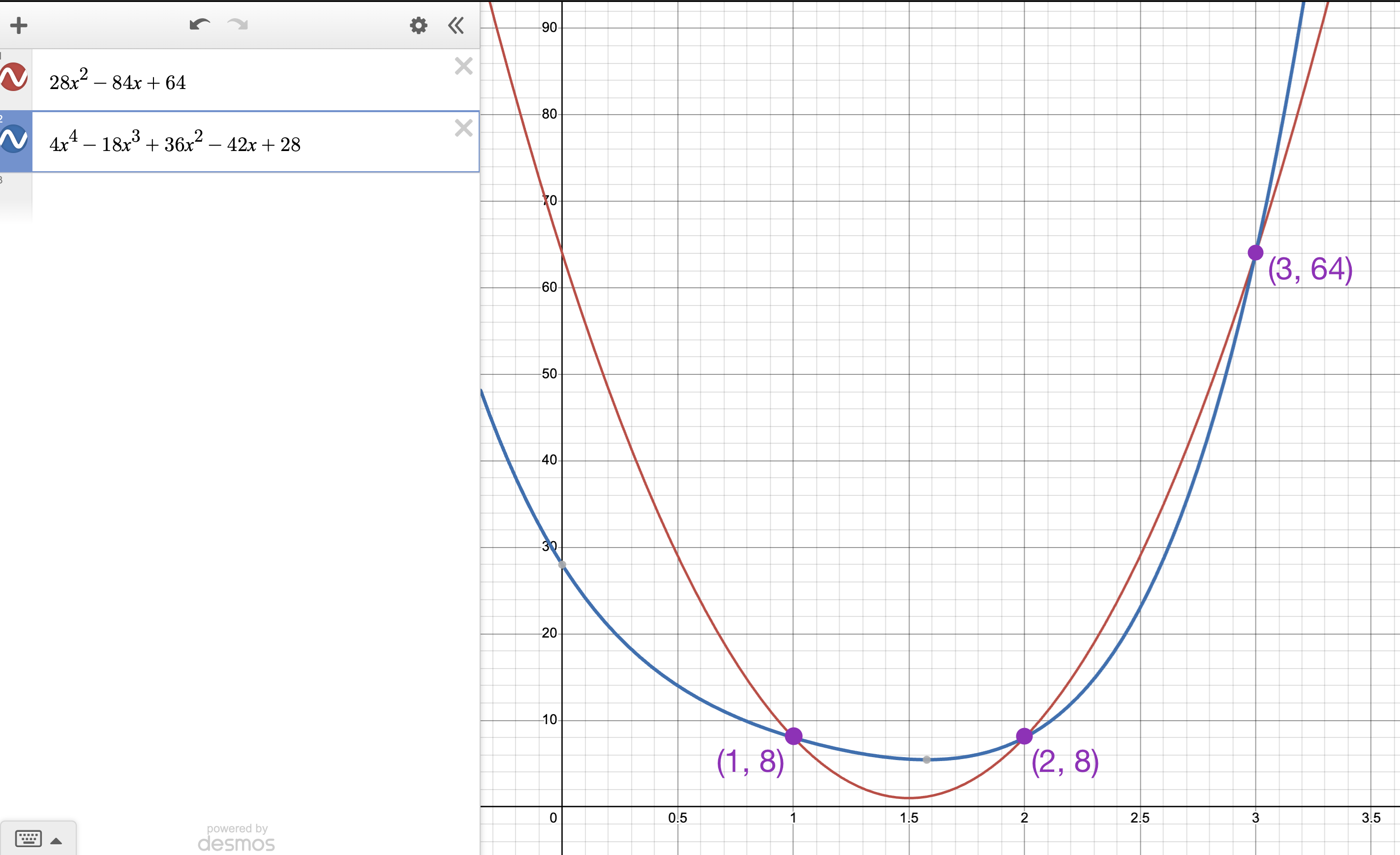
So how can we “make” $w(x)$ equal to $u(x)v(x)$ if they interpolate the same $y$ values over $(1,2,…,n)$?

Interpolating the $\mathbf{0}$ vector

If $\mathbf{v_1} \circ \mathbf{v_2} = \mathbf{v_3}$, then $\mathbf{v_1} \circ \mathbf{v_2} = \mathbf{v_3} + \mathbf{0}$.

Instead of interpolating $\mathbf{0}$ with Lagrange interpolation and getting $f(x) = 0$ (remember Lagrange interpolation finds the lowest degree interpolating polynomial), we can use a higher degree polynomial that will balance out the mismatch in degrees.

For example, the black polynomial ($b(x)$) in the image below interpolates $[(1,0), (2,0), (3,0)]$:

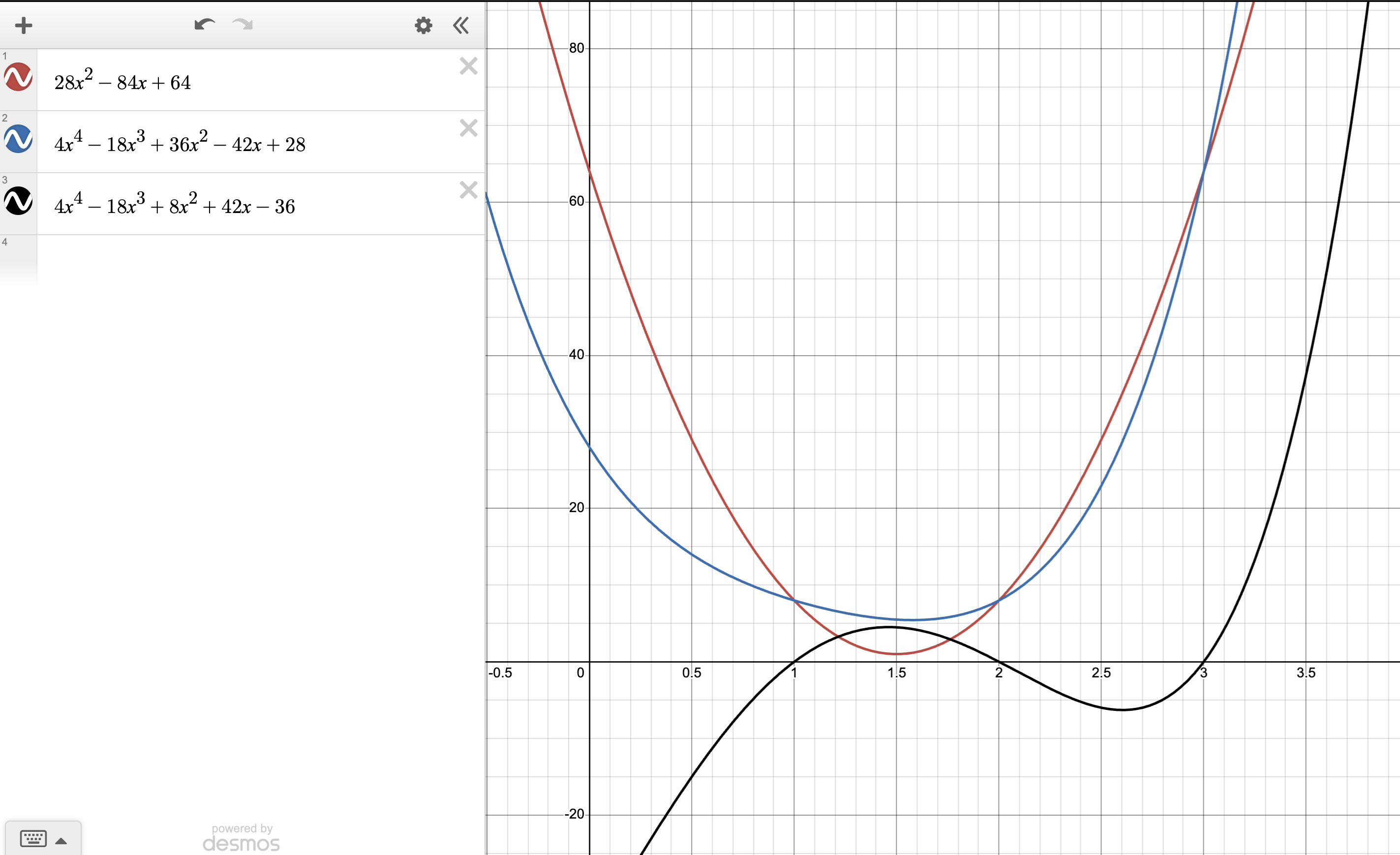
Now, since $4x^4 -18x^3 + 8x^2 + 42x – 36$ is a valid interpolation of $[0,0,0]$, we can write our original

$u(x)v(x) = w(x) + b(x)$

and the equation will be balanced!

$b(x)$ was simply computed as $u(x)v(x) – w(x)$ (the blue polynomial minus red polynomial)

However, we can’t just let the prover pick any $b(x)$, otherwise they could pick a $b(x)$ that balances $u(x)v(x)$ and $w(x)$ even if they do not interpolate the same vector ($[8, 8, 64]$ in our example). The prover has too much flexibility in choosing $b(x)$. Specifically, we want to require $b(x)$ to have roots at $x = 1,2,\dots,n$ — that is, to interpolate the $\mathbf{0}$ vector. That way, the polynomial transformation of $\mathbf{v}_1 \circ \mathbf{v}_2 = \mathbf{v}_3 + \mathbf{0}$ still respects the underlying vectors.

To restrict their choice of $b(x)$, we can use the following theorem:

The union of roots of the polynomial product

Theorem: If $h(x) = f(x)g(x)$ and $f(x)$ has set of roots $\set{r_f}$ and $g(x)$ has set of roots $\set{r_g}$, then $h(x)$ has roots $\set{r_f} \cup \set{r_g}$.

Example

Let $f(x) = (x – 3)(x – 4)$ and $g(x) = (x – 5)(x – 6)$. Then $h(x) = f(x)g(x)$ has roots $\set{3,4,5,6}$.

We can use the theorem above to enforce that $b(x)$ has roots at $x = 1,2,\dots,n$.

Forcing $b(x)$ to be the zero vector

We decompose $b(x)$ into $b(x) = h(x)t(x)$ where $t(x)$ is the polynomial

$$ t(x) = (x-1)(x-2)\dots(x-n) $$

then any polynomial multiplied with $t(x)$ will also be the zero vector, as it must have roots at $x = 1,2,\dots,n$.

Therefore, we will replace $b(x)$ with $h(x)t(x)$ in our equation.

Thus, our equality will become

$$ u(x)v(x) = w(x) + h(x)t(x) $$

We can compute $h(x)$ using basic algebra:

$$ h(x) = \frac{u(x)v(x) – w(x)}{t(x)} $$

QAP End-to-end

Suppose we have an R1CS with matrices $\mathbf{L}$, $\mathbf{R}$, and $\mathbf{O}$ and witness vector $\mathbf{a}$.

$$\mathbf{L}\mathbf{a}\circ\mathbf{R}\mathbf{a} = \mathbf{O}\mathbf{a}$$

The matrices have $n$ columns and $m$ rows where $n = 3$ and $m = 4$.

That is, $\mathbf{L}$, $\mathbf{R}$, and $\mathbf{O}$ are as follows:

$$ \begin{array}{c} \mathbf{L} = \begin{bmatrix} \quad l_{11} \quad& l_{12} \quad& l_{13} \quad& l_{14} \quad\\ \quad l_{21} \quad& l_{22} \quad& l_{23} \quad& l_{24} \quad\\ \quad l_{31} \quad& l_{32} \quad& l_{33} \quad& l_{34} \quad \end{bmatrix} \\ \\ \mathbf{R} = \begin{bmatrix} \quad r_{11} \quad& r_{12} \quad& r_{13} \quad& r_{14} \quad\\ \quad r_{21} \quad& r_{22} \quad& r_{23} \quad& r_{24} \quad\\ \quad r_{31} \quad& r_{32} \quad& r_{33} \quad& r_{34} \quad \end{bmatrix} \\ \\ \mathbf{O} = \begin{bmatrix} \quad o_{11} \quad& o_{12} \quad& o_{13} \quad& o_{14} \quad\\ \quad o_{21} \quad& o_{22} \quad& o_{23} \quad& o_{24} \quad\\ \quad o_{31} \quad& o_{32} \quad& o_{33} \quad& o_{34} \quad \end{bmatrix} \end{array} $$

And witness vector $\mathbf{a}$ is

$$\mathbf{a} = \begin{bmatrix} a_1 \\ a_2 \\ a_3 \\ a_4 \end{bmatrix}$$

We split each of the matrices into $m$ column vectors and interpolate them on $(1, 2, …, n)$ to produce $m$ polynomials each.

$$ \begin{array}{c} \mathbf{L} = \underbrace{\begin{bmatrix} l_{11} \\l_{12} \\ l_{13} \\ l_{14} \\ \end{bmatrix}}_{u_1(x)} \quad \underbrace{\begin{bmatrix} l_{21} \\ l_{22} \\ l_{23} \\ l_{24} \end{bmatrix}}_{u_2(x)} \quad \underbrace{\begin{bmatrix} l_{31} \\ l_{32} \\ l_{33} \\ l_{34} \\ \end{bmatrix}}_{u_3(x)} \quad \underbrace{\begin{bmatrix} l_{41} \\ l_{42} \\ l_{43} \\ l_{44} \end{bmatrix}}_{u_4(x)} \end{array} $$

$$ \begin{array}{c} \mathbf{R} = \underbrace{\begin{bmatrix} r_{11} \\r_{12} \\ r_{13} \\ r_{14} \\ \end{bmatrix}}_{v_1(x)} \quad \underbrace{\begin{bmatrix} r_{21} \\ r_{22} \\ r_{23} \\ r_{24} \end{bmatrix}}_{v_2(x)} \quad \underbrace{\begin{bmatrix} r_{31} \\ r_{32} \\ r_{33} \\ r_{34} \\ \end{bmatrix}}_{v_3(x)} \quad \underbrace{\begin{bmatrix} r_{41} \\ r_{42} \\ r_{43} \\ r_{44} \end{bmatrix}}_{v_4(x)} \end{array} $$

$$ \begin{array}{c} \mathbf{O} = \underbrace{\begin{bmatrix} o_{11} \\o_{12} \\ o_{13} \\ o_{14} \\ \end{bmatrix}}_{w_1(x)} \quad \underbrace{\begin{bmatrix} o_{21} \\ o_{22} \\ o_{23} \\ o_{24} \end{bmatrix}}_{w_2(x)} \quad \underbrace{\begin{bmatrix} o_{31} \\ o_{32} \\ o_{33} \\ o_{34} \\ \end{bmatrix}}_{w_3(x)} \quad \underbrace{\begin{bmatrix} o_{41} \\ o_{42} \\ o_{43} \\ o_{44} \end{bmatrix}}_{w_4(x)} \end{array} $$

Each of the matrix-vector products $\mathbf{L}\mathbf{a}$, $\mathbf{R}\mathbf{a}$, and $\mathbf{O}\mathbf{a}$ are homorphically equivalent the following polynomials:

$$ \begin{align*} \sum_{i=1}^4 a_iu_i(x) &= a_1u_1(x) + a_2u_2(x) + a_3u_3(x) + a_4u_4(x) = u(x) \\ \sum_{i=1}^m a_iv_i(x) &= a_1v_1(x) + a_2v_2(x) + a_3v_3(x) + a_4v_4(x) = v(x) \\ \sum_{i=1}^m a_iw_i(x) &= a_1w_1(x) + a_2w_2(x) + a_3w_3(x) + a_4w_4(x) = w(x) \\ \end{align*} $$

In our case, $t(x)$ will be

$$t(x) = (x – 1)(x – 2)(x – 3)$$

and $h(x)$ will be

$$h(x) = \frac{u(x)v(x) – w(x)}{t(x)}$$

The final formula for a QAP representation of the original R1CS is

$$\sum_{i=1}^4 a_iu_i(x)\sum_{i=1}^4 a_iv_i(x) = \sum_{i=1}^4 a_iw_i(x) + h(x)t(x)$$

Final formula for a QAP

A QAP is the following formula:

$$\sum_{i=1}^m a_iu_i(x)\sum_{i=1}^m a_iv_i(x) = \sum_{i=1}^m a_iw_i(x) + h(x)t(x)$$

Where $u_i(x)$, $v_i(x)$, and $w_i(x)$ are polynomials that interpolate the columns of $\mathbf{L}$, $\mathbf{R}$, and $\mathbf{O}$ respectively, $t(x)$ is $(x – 1)(x – 2)…(x – n)$, where $n$ is the number of rows in $\mathbf{L}$, $\mathbf{R}$, and $\mathbf{O}$, and $h(x)$ is

$$ h(x) = \frac{\sum_{i=1}^ma_iu_i(x)\sum_{i=1}^ma_iv_i(x) – \sum_{i=1}^ma_iw_i(x)}{t(x)} $$

Succinct zero knowledge proofs with Quadratic Arithmetic Programs

Suppose we had a way for the verifier to send a random value $\tau$ to the prover and the prover would respond with

$$ \begin{align*} A &= u(\tau)\\ B &= v(\tau)\\ C &= w(\tau) + h(\tau)t(\tau) \end{align*} $$

The verifier could check that $AB = C$ and accept that the prover has a valid witness $\mathbf{a}$ that satisfies both the R1CS and the QAP.

However, this would require the verifier to trust that the prover is evaluating the polynomials correctly, and we don’t have a mechanism to force the prover to do so.

In the next chapter, we will show Python code to convert an R1CS to a QAP based on our discussion in this chapter.

Then we will discuss trusted setups to begin to tackle the problem of how to get the prover to evaluate the polynomials honestly.

Originally published August 23, 2023