get_D() and get_y() in Curve StableSwap

Last updated on Aug 20, 2025

This article shows algebraically step-by-step how the code for get_D() and get_y() are derived from the StableSwap invariant.

Given the StableSwap Invariant:

A n^{n} \sum x_{i} + D = A n^{n} D + \frac{D^{n + 1}}{n^{n} \prod x_{i}}

There are two frequent math operations we wish to conduct with it:

Compute $D$ given fixed values for $A$ , and the reserves $x_{1}, \dots, x_{n}$ . Note that $n$ , the number of coins the pool supports, is fixed at the time the pool is deployed. This is what the function get_D() does.
Given $D$ , we wish to increase the value of one of the reserves $x_{i}$ to a new value $x_{i}^{'}$ and figure out how much another reserve $x_{j}$ needs to decrease to keep the equation balanced. This is what the function get_y() does. Here “y” means $x_{i}^{'}$ .

These operations are called get_D() and get_y(), respectively, in Curve StableSwap.

The objective of `get_D()`

In Curve V1 (StableSwap), D behaves similarly to k in Uniswap V2 — the larger D is, the more the reserves are, and the “further out” the price curve will be. D changes — and needs to be recomputed — after liquidity is added or removed, or a fee changes the pool balance. This is what the function get_D() is for. Given the current reserves of the pool, it computes D.

If a curve pool holds two tokens, x and y, the StableSwap invariant is

4 A (x + y) + D = 4 A D + \frac{D^{3}}{4 x y}

The “amplification factor” A, for our purposes, can be treated as a constant.

The objective of `get_y()`

The function get_y() is used during a swap. Similar to k in Uniswap V2, D must be held constant during a swap (ignoring fees). Specifically, given a new value for x, it computes the value of y that keeps the equation balanced. Thus, it is an important subroutine for figuring out “if I put in this much token x into the pool, how much token y can be taken out?”

Curve can hold more than 2 tokens in the pool (e.g. 3pool holds USDT, USDC, and DAI). Curve identifies the coins by an index in an array. So, in this case, x and y refer to particular coins in that array. In this context, get_y() means changing the balance of a particular token x, holding the other balances constant, but allowing another token y to change in value. Then, given a particular change in x, compute how y changes to keep the invariant balanced.

The invariant for n tokens is:

A n^{n} \sum x_{i} + D = A n^{n} D + \frac{D^{n + 1}}{n^{n} \prod x_{i}}

For simplicity, we will use $S$ instead of summation and $P$ instead of product in the rest of the article, so the invariant becomes:

A n^{n} S + D = A D n^{n} + \frac{D^{n + 1}}{n^{n} P}

Where $S$ is the sum of the balances of the tokens ( $x_{0} + x_{1} + \dots + x_{n}$ ), $P$ is the product of the balances ( $x_{0} x_{1} . . . x_{n})$ , and $x_{i}$ is the balance of token i.

In the whitepaper, $S$ is written as $\sum x_{i}$ and $P$ is written as $\prod x_{i}$ . The whitepaper equation is replicated below:

A n^{n} \sum x_{i} + D = A D n^{n} + \frac{D^{n + 1}}{n^{n} \prod x_{i}}

We will use $S$ and $P$ instead of the sum and product notation.

We assume that the pools can hold an arbitrary number $n$ tokens, so the formulas will reflect that. In practice, however, $n$ must be small, otherwise the $D^{n + 1}$ term is liable to overflow.

Computing $D$ with `get_D()`

In get_D(), we are presented with a set of balances x_0, x_1, ..., x_n and we are to compute D.

It is not possible to algebraically solve

A n^{n} S + D = A D n^{n} + \frac{D^{n + 1}}{n^{n} P}

for $D$ . Instead, we need to apply Newton’s method to solve it numerically. To do so, we create a function $f (D)$ , which is 0 when the equation is balanced.

0 = A D n^{n} + \frac{D^{n + 1}}{n^{n} P} - D - A n^{n} S

0 = \frac{D^{n + 1}}{n^{n} P} + A D n^{n} - D - A n^{n} S

f (D) = \frac{D^{n + 1}}{n^{n} P} + A n^{n} D - D - A n^{n} S

and we compute the derivative $f^{'} (D)$ with respect to $D$ as:

f^{'} (D) = \frac{(n + 1) D^{n}}{n^{n} P} + A n^{n} - 1

Newton’s Method Formula

We can iteratively solve for $D$ using:

D_{next} = D - \frac{f (D)}{f^{'} (D)}

It will be helpful to express $f^{'} (D)$ with $D$ in the denominator. First we multiply the top and bottom of the left fraction defining $f^{'} (D)$ by $D$ .

f^{'} (D) = \frac{\frac{(n + 1) D^{n + 1}}{n^{n} P}}{D} + A n^{n} - 1

And then combine $f^{'} (D)$ into a single fraction:

\begin{matrix} f^{'} (D) & = \frac{\frac{(n + 1) D^{n + 1}}{n^{n} P}}{D} + \frac{(A n^{n} - 1) D}{D} \\ f^{'} (D) & = \frac{\frac{(n + 1) D^{n + 1}}{n^{n} P} + (A n^{n} - 1) D}{D} \end{matrix}

We can re-write Newton’s method to have a common denominator:

\begin{matrix} D_{next} & = D - \frac{f (D)}{f^{'} (D)} & // Newton’s Method \\ = D \frac{f^{'} (D)}{f^{'} (D)} - \frac{f (D)}{f^{'} (D)} & // multiply D by \frac{f^{'} (D)}{f^{'} (D)} \\ = \frac{D f^{'} (D) - f (D)}{f^{'} (D)} & // combine by common denominator \end{matrix}

By substituting the $f (D)$ and $f^{'} (D)$ from earlier into the re-written Newton’s method formula we get:

= \frac{D \frac{(n + 1) \frac{D^{n + 1}}{n^{n} P} + (A n^{n} - 1) D}{D} - (\frac{D^{n + 1}}{n^{n} P} + A n^{n} D - D - A n^{n} S)}{\frac{(n + 1) \frac{D^{n + 1}}{n^{n} P} + (A n^{n} - 1) D}{D}}

Since we re-arranged $f^{'} (D)$ to have $D$ in the denominator, the $D f^{'} (D)$ term will cancel nicely:

= \frac{D \frac{(n + 1) \frac{D^{n + 1}}{n^{n} P} + (A n^{n} - 1) D}{D} - (\frac{D^{n + 1}}{n^{n} P} + A n^{n} D - D - A n^{n} S)}{\frac{(n + 1) \frac{D^{n + 1}}{n^{n} P} + (A n^{n} - 1) D}{D}}

= \frac{(n + 1) \frac{D^{n + 1}}{n^{n} P} + (A n^{n} - 1) D - (\frac{D^{n + 1}}{n^{n} P} + A n^{n} D - D - A n^{n} S)}{\frac{(n + 1) \frac{D^{n + 1}}{n^{n} P} + (A n^{n} - 1) D}{D}}

Distribute all the terms to remove the parenthesis in the numerator:

= \frac{\frac{D^{n + 1}}{n^{n} P} + \frac{n D^{n + 1}}{n^{n} P} + A n^{n} D - D - \frac{D^{n + 1}}{n^{n} P} - A n^{n} D + D + A n^{n} S}{\frac{(n + 1) \frac{D^{n + 1}}{n^{n} P} + (A n^{n} - 1) D}{D}}

This leads to a lot of cancellations

= \frac{\frac{D^{n + 1}}{n^{n} P} + \frac{n D^{n + 1}}{n^{n} P} + A n^{n} D - D - \frac{D^{n + 1}}{n^{n} P} - A n^{n} D + D + A n^{n} S}{\frac{(n + 1) \frac{D^{n + 1}}{n^{n} P} + (A n^{n} - 1) D}{D}}

= \frac{\frac{n D^{n + 1}}{n^{n} P} + A n^{n} S}{\frac{(n + 1) \frac{D^{n + 1}}{n^{n} P} + (A n^{n} - 1) D}{D}}

We multiply the numerator and denominator by $D$

= \frac{(A n^{n} S + n \frac{D^{n + 1}}{n^{n} P}) D}{(A n^{n} - 1) D + (n + 1) \frac{D^{n + 1}}{n^{n} P}}

If we define $D_{p}$ as

D_{p} = \frac{D^{n + 1}}{n^{n} P}

and substitute $D_{p}$ we get

= \frac{(A n^{n} S + n \frac{D^{n + 1}}{n^{n} P}) D}{(A n^{n} - 1) D + (n + 1) \frac{D^{n + 1}}{n^{n} P}}

D_{next} = \frac{(A n^{n} S + D_{p} n) D}{(A n^{n} - 1) D + (n + 1) D_{p}}

Comparison to the original source code

This matches exactly what is in the Vyper code:

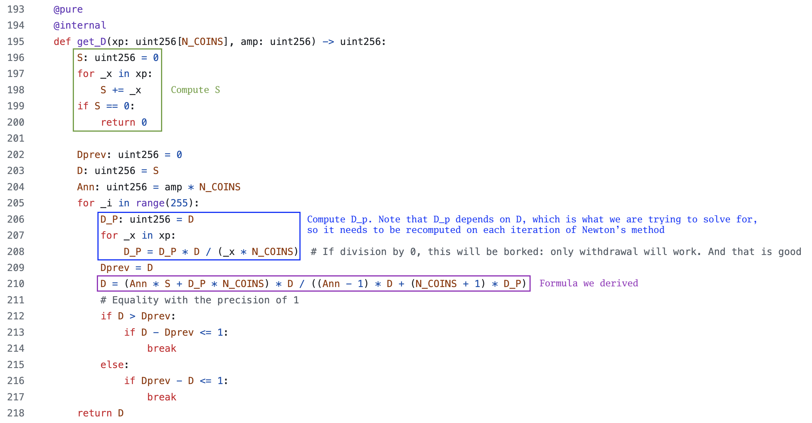
The variable $D_{p}$ was defined as:

D_P: uint256 = D # D_P = S

for _x in xp:
    D_P = D_P * D / (_x * N_COINS)

xp is the number of tokens, so the loop will run n times. Therefore, we have $D$ multiplied by itself n times in the denominator

D_{p} = \frac{D^{n + 1}}{n^{n} \prod_{i = 1}^{n} x_{i}}

Computing `y` with `get_y()`

The idea is we force one of the $x_{i}$ to take on a new value (the code calls this x) and calculate the correct value for another $x_{j}$ (where $i \neq j)$ such that the equation stays balanced. The balance of the other tokens remains unchanged. $x_{j}$ is referred to as $y$ .

Although a StableSwap pool could have multiple tokens, it is only possible to exchange two of those tokens at a time using get_y().

Again, we have the same invariant

A n^{n} S + D = A D n^{n} + \frac{D^{n + 1}}{n^{n} P}

$D$ , $A$ , and $n$ are fixed, but we will be changing two of the values in $S$ and $P$

\begin{matrix} S & = x_{0} + x_{1} + . . . + x_{n} \\ P & = x_{0} x_{1} . . . x_{n} \end{matrix}

Therefore, we need to adjust the formula a bit, since $S$ and $P$ contain the values we are computing for.

$S^{'}$ will be the sum of all the balances except the new balance of token $x_{i}$ that we are trying to solve for
$P$ will be the product of the balances of all the tokens, except for the one we are trying to solve for.

In other words,

\begin{matrix} S & = S^{'} + y \\ P & = P^{'} y \end{matrix}

To stay consistent with the code, we will call the token whose new balance we are trying to compute $y$ .

The formula then becomes

A n^{n} (S^{'} + y) + D = A D n^{n} + \frac{D^{n + 1}}{n^{n} P^{'} y}

Again, we derive an $f (y)$ which is 0 when the equation is balanced, and its derivative with respect to y

\begin{matrix} f (y) & = A D n^{n} + \frac{D^{n + 1}}{n^{n} P^{'} y} - A n^{n} (S^{'} + y) - D \\ f^{'} (y) & = \frac{- D^{n + 1}}{n^{n} P^{'} y^{2}} - A n^{n} \end{matrix}

Here is the formula for Newton’s method again:

y_{next} = y - \frac{f (y)}{f^{'} (y)}

After substituting $f (y)$ and $f^{'} (y)$ into Newton’s method we get:

y_{next} = y - \frac{A D n^{n} + \frac{D^{n + 1}}{n^{n} P^{'} y} - A n^{n} (S^{'} + y) - D}{\frac{- D^{n + 1}}{n^{n} P^{'} y^{2}} - A n^{n}}

Take $- 1$ out of the denominator

y_{next} = y - - 1 \cdot \frac{A D n^{n} + \frac{D^{n + 1}}{n^{n} P^{'} y} - A n^{n} (S^{'} + y) - D}{\frac{D^{n + 1}}{n^{n} P^{'} y^{2}} + A n^{n}}

y_{next} = y + \frac{A D n^{n} + \frac{D^{n + 1}}{n^{n} P^{'} y} - A n^{n} (S^{'} + y) - D}{\frac{D^{n + 1}}{n^{n} P^{'} y^{2}} + A n^{n}}

Multiply $y$ (in the box below) to have a common denominator:

y_{next} = y + \frac{A D n^{n} + \frac{D^{n + 1}}{n^{n} P^{'} y} - A n^{n} (S^{'} + y) - D}{\frac{D^{n + 1}}{n^{n} P^{'} y^{2}} + A n^{n}}

y_{next} = y \frac{\frac{D^{n + 1}}{n^{n} P^{'} y^{2}} + A n^{n}}{\frac{D^{n + 1}}{n^{n} P^{'} y^{2}} + A n^{n}} + \frac{A D n^{n} + \frac{D^{n + 1}}{n^{n} P^{'} y} - A n^{n} (S^{'} + y) - D}{\frac{D^{n + 1}}{n^{n} P^{'} y^{2}} + A n^{n}}

Distribute $y$ in the left term

y_{next} = y \frac{\frac{D^{n + 1}}{n^{n} P^{'} y^{2}} + A n^{n}}{\frac{D^{n + 1}}{n^{n} P^{'} y^{2}} + A n^{n}} + \frac{A D n^{n} + \frac{D^{n + 1}}{n^{n} P^{'} y} - A n^{n} (S^{'} + y) - D}{\frac{D^{n + 1}}{n^{n} P^{'} y^{2}} + A n^{n}}

y_{next} = \frac{\frac{D^{n + 1}}{n^{n} P^{'} y} + A n^{n} y}{\frac{D^{n + 1}}{n^{n} P^{'} y^{2}} + A n^{n}} + \frac{A D n^{n} + \frac{D^{n + 1}}{n^{n} P^{'} y} - A n^{n} S^{'} - A n^{n} y - D}{\frac{D^{n + 1}}{n^{n} P^{'} y^{2}} + A n^{n}}

Combine the sums with a common denominator

y_{next} = \frac{A D n^{n} + 2 \frac{D^{n + 1}}{n^{n} P^{'} y} - A n^{n} S^{'} - D}{\frac{D^{n + 1}}{n^{n} P^{'} y^{2}} + A n^{n}}

Creating a substitution from the original invariant

It might seem like the equation cannot be simplified further, but if we revisit our original invariant

A n^{n} (S^{'} + y) + D = A D n^{n} + \frac{D^{n + 1}}{n^{n} P^{'} y}

We can solve for $A D n^{n}$ we get

A n^{n} (S^{'} + y) + D = A D n^{n} + \frac{D^{n + 1}}{n^{n} P^{'} y}

A n^{n} (S^{'} + y) + D - \frac{D^{n + 1}}{n^{n} P^{'} y} = A D n^{n}

A D n^{n} = - \frac{D^{n + 1}}{n^{n} P^{'} y} + A n^{n} (S^{'} + y) + D

And then if we substitute $A D n^{n}$ into the numerator in our latest formula for $y_{next}$ , we get

y_{next} = \frac{A D n^{n} + 2 \frac{D^{n + 1}}{n^{n} P^{'} y} - A n^{n} S^{'} - D}{\frac{D^{n + 1}}{n^{n} P^{'} y^{2}} + A n^{n}}

y_{next} = \frac{(- \frac{D^{n + 1}}{n^{n} P^{'} y} + A n^{n} (S^{'} + y) + D) + 2 \frac{D^{n + 1}}{n^{n} P^{'} y} - A n^{n} S^{'} - D}{\frac{D^{n + 1}}{n^{n} P^{'} y^{2}} + A n^{n}}

A lot of cancellation happens

y_{next} = \frac{- \frac{D^{n + 1}}{n^{n} P^{'} y} + A n^{n} S^{'} + A n^{n} y + D + 2 \frac{D^{n + 1}}{n^{n} P^{'} y} - A n^{n} S^{'} - D}{\frac{D^{n + 1}}{n^{n} P^{'} y^{2}} + A n^{n}}

And we are left with a much smaller equation

y_{next} = \frac{A n^{n} y + \frac{D^{n + 1}}{n^{n} P^{'} y}}{\frac{D^{n + 1}}{n^{n} P^{'} y^{2}} + A n^{n}}

We multiply the top and bottom by $\frac{y}{A n^{n}}$

y_{next} = \frac{(A n^{n} y + \frac{D^{n + 1}}{n^{n} P^{'} y}) \frac{y}{A n^{n}}}{(\frac{D^{n + 1}}{n^{n} P^{'} y^{2}} + A n^{n}) \frac{y}{A n^{n}}}

y_{next} = \frac{y^{2} + \frac{D^{n + 1}}{n^{n} P^{'} A n^{n}}}{\frac{D^{n + 1}}{n^{n} P^{'} y} \frac{1}{A n^{n}} + y}

Going back to our invariant, we can solve for the fractional term in the denominator:

A n^{n} (S^{'} + y) + D = A D n^{n} + \frac{D^{n + 1}}{n^{n} P^{'} y}

\frac{D^{n + 1}}{n^{n} P^{'} y} = A n^{n} (S^{'} + y) + D - A D n^{n}

Then we can substitute that into the equation for ynext:

y_{next} = \frac{y^{2} + \frac{D^{n + 1}}{n^{n} P^{'} A n^{n}}}{\frac{D^{n + 1}}{n^{n} P^{'} y} \frac{1}{A n^{n}} + y}

y_{next} = \frac{y^{2} + \frac{D^{n + 1}}{n^{n} P^{'} A n^{n}}}{(A n^{n} (S^{'} + y) + D - A D n^{n}) \frac{1}{A n^{n}} + y}

Then we can distribute $\frac{1}{A n^{n}}$ and simplify the denominator

y_{next} = \frac{y^{2} + \frac{D^{n + 1}}{n^{n} P^{'} A n^{n}}}{((S^{'} + y) + \frac{D}{A n^{n}} - D) + y}

y_{next} = \frac{y^{2} + \frac{D^{n + 1}}{n^{n} P^{'} A n^{n}}}{(S^{'} + y + \frac{D}{A n^{n}} - D) + y}

Simplify the denominator by removing the parenthesis and adding the two $y$ together

y_{next} = \frac{y^{2} + \frac{D^{n + 1}}{n^{n} P^{'} A n^{n}}}{2 y + S^{'} + \frac{D}{A n^{n}} - D}

In the original code, Curve defines additional variables:

c = \frac{D^{n + 1}}{n^{n} P^{'} A n^{n}}

b = S^{'} + \frac{D}{A n^{n}}

After substitution into the formula for $y_{next}$ , we get:

y_{next} = \frac{y^{2} + \frac{D^{n + 1}}{n^{n} P^{'} A n^{n}}}{2 y + S^{'} + \frac{D}{A n^{n}} - D}

y_{next} = \frac{y^{2} + c}{2 y + b - D}

Comparison to the original source code

This matches the Curve code exactly, see the purple box below:

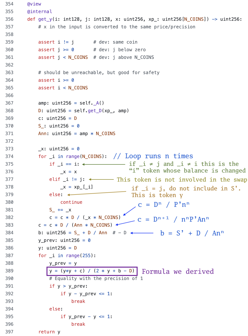
Mismatch between Ann and Anⁿ

Rather confusingly, the Curve whitepaper uses the invariant $A n^{n}$ but the codebase uses $A n n$ . That is, the codebase appears to be computing A * n * n rather than A * n ** n. The reason for this discrepancy is that the codebase stores $A$ as $A n^{n - 1}$ . Since $n$ is fixed at deployment time, precomputing $n^{n - 1}$ allows the code to avoid computing an exponent on-chain, which is more costly operation.

Summary

The core invariant of the Curve does not allow the variables $D$ or $x_{i}$ to be solved symbolically. Instead, the terms must be solved numerically.

One takeway from this exercise is that good algebraic manipulation is a very effective gas optimization technique. The Curve developers were able to compute Newton’s method formula that is much smaller than naively plugging in $f$ and its derivative and leaving it at that.

Citations and Acknowledgements

The following resources were consulted in writing this article:

StableSwap - efficient mechanism for Stablecoin liquidity, Michael Egorov, https://resources.curve.fi/pdf/curve-stableswap.pdf

Understanding the Curve AMM, Part -1: StableSwap Invariant, Atul Agarwal https://atulagarwal.dev/posts/curveamm/stableswap/

Curve Finance Discord, “chanho”

https://discord.com/channels/729808684359876718/729812922649542758/1126630568004698132

Curve - Code Explaind - get_y() | DeFi, Smart Contract Programmer https://www.youtube.com/watch?v=jAhKbxoeskQ

get_D() and get_y() in Curve StableSwap

The objective of get_D()

The objective of get_y()

Computing D with get_D()

Newton’s Method Formula

Comparison to the original source code

Computing y with get_y()

Creating a substitution from the original invariant

Comparison to the original source code

Mismatch between Ann and Anⁿ

Summary

Citations and Acknowledgements

The objective of `get_D()`

The objective of `get_y()`

Computing $D$ with `get_D()`

Computing `y` with `get_y()`