This article explains how Uniswap V3 implements concentrated liquidity. We assume the reader already understands Uniswap V2.
To understand concentrated liquidity, we first need to precisely define liquidity, which itself depends on understanding the reserves.
Reserve
The reserve of a token is the balance of a specific tradeable token held by an automated market maker (AMM). We use or simply to refer to the amount of tradeable token held by the pool, and (or sometimes ) to refer to the amount of tradeable token held by the pool.
Liquidity
Liquidity, in the context of AMMs, measures the combined reserves of the token pair and .
Liquidity providers (LPs) provide liquidity when they deposit tokens into the pool in hopes of earning fees during swaps. Their deposit increases the reserves, which in turn, increases the liquidity.
Liquidity is a function of the reserves. It is often the product, the square of the product, or some other monotonically increasing function of the reserves (a monotonically increasing function is a function that always increases if the input increases).
In Uniswap V2, the liquidity is measured as the in (the product of the reserves).
There can be different combinations of the reserves, but the liquidity stays the same. For example, if there is 1 ETH and 1000 USDC, then the liquidity is 1000 (1 ETH × 1000 USDC = 1000, ignoring decimals).
If there was 900 USDC and 1.1111 ETH, the liquidity remains at 1000 because 900 × 1.1111 = 1000.
The following animation plots , while sweeping the value for . Note that as gets larger, the curve moves further away from the origin.
The more reserves there are, the greater the distance of the curve from the origin, and the greater the liquidity.
Because the fees paid by the traders are absorbed into the reserves in Uniswap V2, Uniswap V2 uses the invariant , not . To keep the math simple, we ignore fees in this article.
Liquidity and Price Impact
High liquidity is desirable because traders can “swap out” more of a token. If a pool only holds 1000 USDC, it is impossible for a trader to swap out more than 1000 USDC. But even if they don’t need to use up all the reserves of a particular token, traders still prefer higher liquidity because higher liquidity reduces price impact.
To precisely define “price impact” we first need to precisely define “price” in an AMM.
Price of an asset in an AMM
The price of token0 in Uniswap V2 is calculated using the following formula:
In Uniswap v3, tokens X and Y are also known as token0 and token1. In these chapters, we will use both notations interchangeably.
Below we show a regular price curve. The green point on the curve represents the current reserves of both token0 and token1. Recall that we are using token0 and token X to refer to the same thing (and same for token1 and token Y). As the green point moves up and to the left, the price of token0 increases, as that corresponds to smaller reserves of token0:
As can be seen in the graphic above and in the formula:
reducing the reserve of token0 causes its price to increase. This matches the law of supply and demand, since the more scarce token0 is, the higher its price.
Price as the angle from the origin
We can visualize “price” as a ray (a line with a starting point, but no end point) from the origin. The ray represents a certain fixed ratio of reserves, regardless of the liquidity.
Consider that any combination of reserves that intersects with the yellow ray below has the same ratio. Hence, the point of intersection on this ray with the price curve represents the same price, regardless of the liquidity:
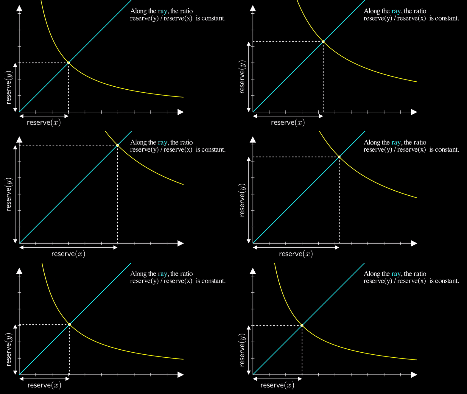
Let be the angle of the ray from the origin to the current price on the price curve. The greater the angle of , the higher the price:
Now that we have a rigorous definition and visualization of price, we can define and illustrate price impact. We will tie price impact back to liquidity afterwards.
Price Impact
Any trade in an AMM causes the price to move against the trader.
If a trader tries to give token1 to the pool to swap out token0, then token0 will become more expensive.
As seen earlier, AMMs adjust prices based on the supply (reserve) of tokens in the pool. This ensures the price always moves in response to a buy or sell order. The increase in price reflects the increase in demand.
Now we can examine how the price changes in response to a trade.
Price impact of a small order
Let’s say you place the tiniest possible order to buy some token0 by paying token1 to the pool. This causes the reserve of token0 to go slightly down and the reserve of token1 to go slightly up. The price of token0 must go up (a small amount) as a result.
In other words, let the price before the trade be
and after the trade:
where is the amount of token1 the trader paid the pool and is the amount of token0 the trader obtained from the pool.
Amounts and , and their effect on the price, are shown visually below:
Regardless of how small and are (as long as they are not zero), it must be the case that
Therefore, any trade on an AMM, no matter how small, changes the price.
We call the change in price as the result of a trade the price impact.
A large price impact means the price changed significantly and a small price impact means the price changed a tiny amount.
Price impact examples for different liquidity levels
For a trade of a fixed size, the greater the liquidity, the lower the price impact.
This section shows three examples of the same trade (purchasing 1 USDC using USDT) in pools with increasing liquidity levels.
Example 1: xy = 100
Suppose a pool is holding 10 USDC (token0) and 10 USDT (token1). Since , . Therefore, the liquidity is 100.
If a trader wishes to obtain 1 USDC, they must decrease the USDC reserve from 10 USDC to 9 USDC.
They must then put in enough USDT such that 9 * new_reserve_usdt = 100 (ignoring fees). Solving for new_reserve_usdt, we obtain 11.11. Since the original reserve of USDT was 10, the trader must put in 1.11 USDT to obtain 1 USDC. If we look at the price of USDC after the trade, we get:
As a result of buying 1 USDC, the price of USDC went from 1 USDT to 1.234 USDT.
Let’s call the initial price of 1USDT : 1USDC the start price.
The end price is 1.234USDT : 1USDC. The price impact is 0.234, or a 23.4% increase of the original price.
We visualize the price impact of this trade below.
The price starts on the intersection between the dotted green ray and the blue price curve. The green ray is plotted with , since the assets start at the same price. The end price is where the red ray intersects the blue price curve. The price impact is quite visible here (the graph is to scale):
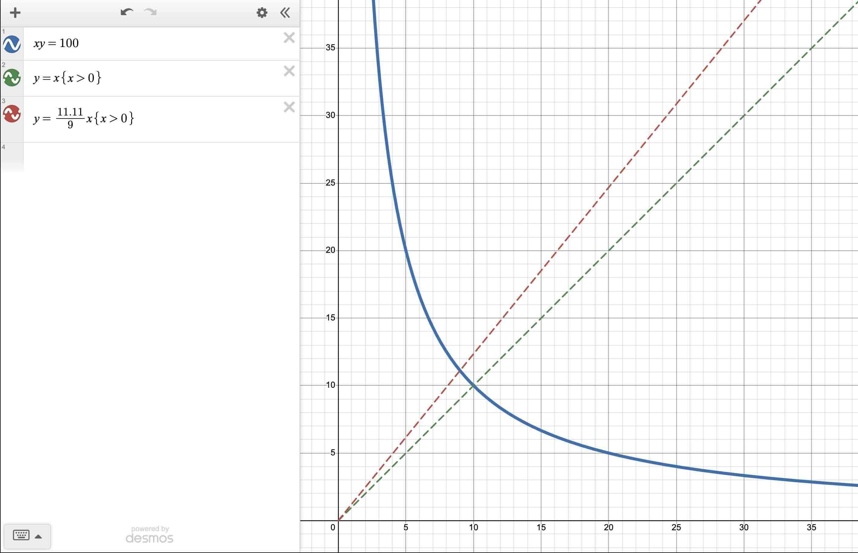
(We assume that both tokens have the same amount of decimals, so the decimals can be ignored).
Example 2: xy = 10,000
Now, suppose the pool holds 100 USDC and 100 USDT. Since , . The liquidity increased 10 times from the previous example.
If a trader wishes to obtain 1 USDC, they must decrease the reserve of USDC from 100 USDC to 99 USDC. They must then put in enough USDT such that 99 * new_reserve_usdt = 10_000. Solving for new_reserve_usdt, we obtain 101.01. Since the original reserve of USDT was 100, the trader must put in 1.01 USDT to obtain 1 USDC. If we look at the price of USDC after the trade, we get:
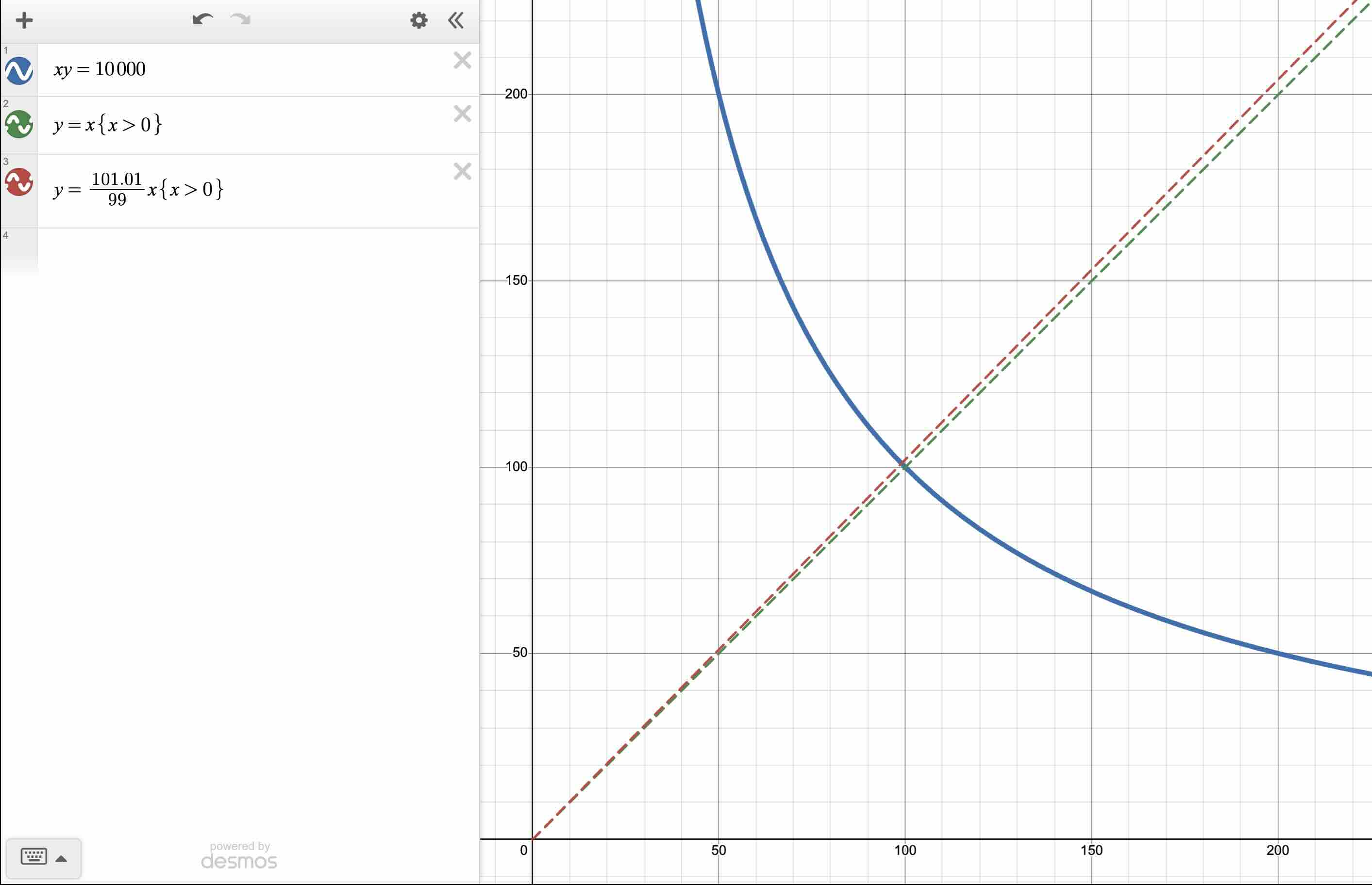
As a result of buying 1 USDC (when the reserves started at 100 USDC and 100 USDT), the price of USDC went from 1 USDT to 1.02 USDT, resulting in 2% increase in price.
In this example and the previous, the trader obtained 1 USDC. However, the price impact in this example is a lot lower (23 cents previously vs 2 cents here). As a byproduct, the price the trader paid for the 1 USDC is smaller, 1.01 USDT, compared to 1.11 USDT in the first example.
When the AMM’s liquidity increases, the price impact decreases.
The price impact in this example is noticeably smaller:
Example 3: xy = 1 quintillion
To drive the point home, let’s suppose the reserves are 1 billion USDC and 1 billion USDT, and the liquidity is 1 quintillion.
We suggest the reader try to solve for the price impact before reading the calculation below.
If a trader wishes to obtain 1 USDC, they must decrease the USDC reserve from 1 billion USDC to 999,999,999 USDC. They must then put in enough USDT such that 999,999,999 * new_reserve_usdt = 1 quintillion (1 billion 1 billion). Solving for new_reserve_usdt, we obtain 1,000,000,001.000000001. Since the original reserve of USDT was 1 billion, the trader must put in 1.000000001 USDT to obtain 1 USDC. If we look at the price of USDC after the trade, we get:
The price of UDSC in terms of USDT increased, but by a very small amount.
Hence, when the liquidity is extremely large relative to the trade size, the price impact is barely noticeable.
Capital Efficient Liquidity
Traders prefer having a small price impact, but liquidity providers do not want to provide a large sum of two billion dollars to accomplish this.
We want to accomplish high liquidity without such a high capital demand.
We want our liquidity to be capital efficient.
To make our liquidity capital efficient, we exploit the fact that we know the “expected” price of the trade. Specifically, both USDC and USDT are pegged to the United States Dollar, so they are expected to trade at 1:1.
However, because of price impact, USDC and USDT do not trade at 1:1 — this is the problem we are trying to minimize. But we want to minimize price impact while also supplying a lot less than two billion dollars in reserves.
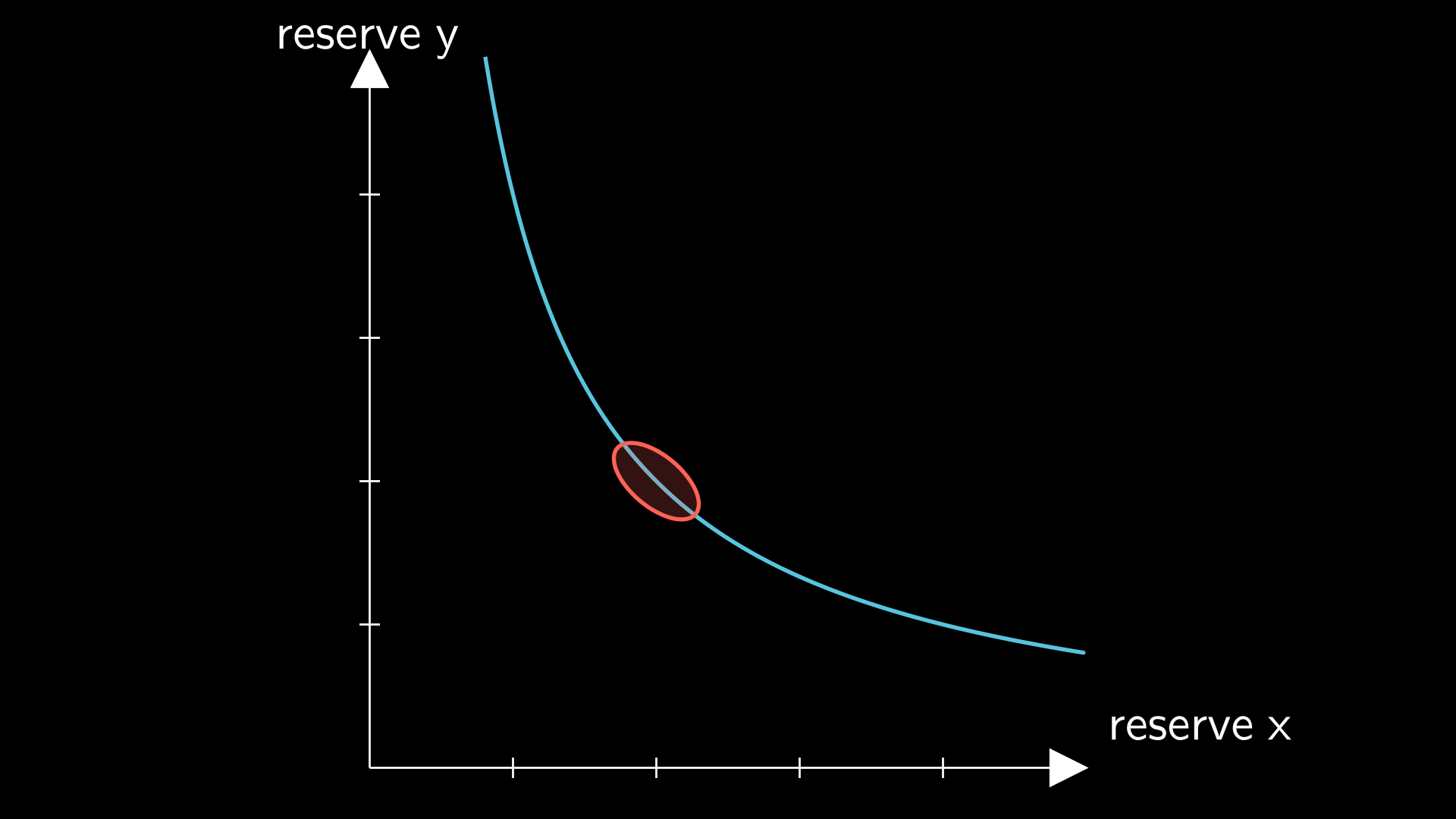
Since we expect the trade price to be 1:1 or close to it, we expect most of the trades to happen in the region where the reserves are equal to each other, as visualized below. If the price goes outside this region, then arbitragers will buy up the cheaper stablecoin and sell it on an exchange. Therefore, we can expect most trades to happen in the red region below:
Wasted liquidity
As modeled in the curve above, Uniswap V2 supports trades in the price range of essentially 0 to infinity. Spreading liquidity out over such wide price range wastes liquidity because most of it will be unused, especially in the case of a stablecoin pair.
It would be better to remove the ability to allow trading at extreme prices in exchange for better liquidity in the region where we expect trades to happen.
Concentrating liquidity
What if we could “remove” liquidity from the regions where we don’t expect trading to happen and add the liquidity into the expected region?
To use concrete numbers as an example, suppose we want our AMM to have high liquidity above the price of 0.99:1 (99 cents of Tether for one USDC) and below the price 1.01:1 (1.01 Tether for one USDC). Recall that price increases as our location on the curve moves up and to the left.
If we put an if statement at those price boundaries, we could have our AMM curve look like the following piecewise function:
If we plot the piecewise equation above, we get the following:
Since we have a much larger liquidity in the price range where we expect the stablecoins to trade, we expect a significantly reduced price in that region. We reduced price impact for most trades without requiring more capital.
Of course, nothing is free. If the price wanders outside the [0.99, 1.01] boundary, then liquidity drops precipitously. To create a competitive pool, we need to set the boundaries optimally. It’s also not obvious that 0.99 and 1.01 are the optimal boundaries. Nor is it obvious that multiplying and dividing the liquidity by a factor of 10 is the right scale.
How Uniswap V3 Implements Concentrated Liquidity
To make things flexible in letting the LPs decide the ideal boundaries and quantity for where to place liquidity, Uniswap V3 doesn’t use a scaling factor at all. Within certain price boundaries, will be the liquidity the LPs provide there. That is, liquidity providers can choose from a variety of price regions where they can provide liquidity.
We noted at the beginning of this article that liquidity is proportional to the distance of the price curve from the origin.
Therefore, since the liquidity varies for different price ranges, the price curve of a Uniswap V3 pool might look like the following graphic.
Even though the curves appear to be discontinuous, the price (represented with the orange ray) can transition smoothly between each “mini Uniswap V2 curve.” Each of the “sub curves” are of the form , but is different for each sub curve. The value of for a sub curve will entirely depend on how much liquidity LPs placed there. As the liquidity for that segment increases, its distance from the origin increases. Since the curves have different liquidities, their distances from the origin varies.
Increasing means the liquidity provider provided the right combination of token and token to push the curve out. In practice, LPs specify a liquidity, and then Uniswap V3 calculates the amount of and the LP needs to provide. The amount of and held by that segment will vary depending on the swaps that happen in that region. For now we don’t have to worry about the amounts of and for each sub curve, only that their product is . This will be discussed more in the following chapters.
To keep accounting simple, LPs cannot provide liquidity at arbitrary price boundaries, but at predefined prices called ticks. Recall that the price is proportional to the angle of a ray from the origin to the price point on the curve. Therefore, we can visualize ticks as places where the price curve intersects with predefined rays from the origin:
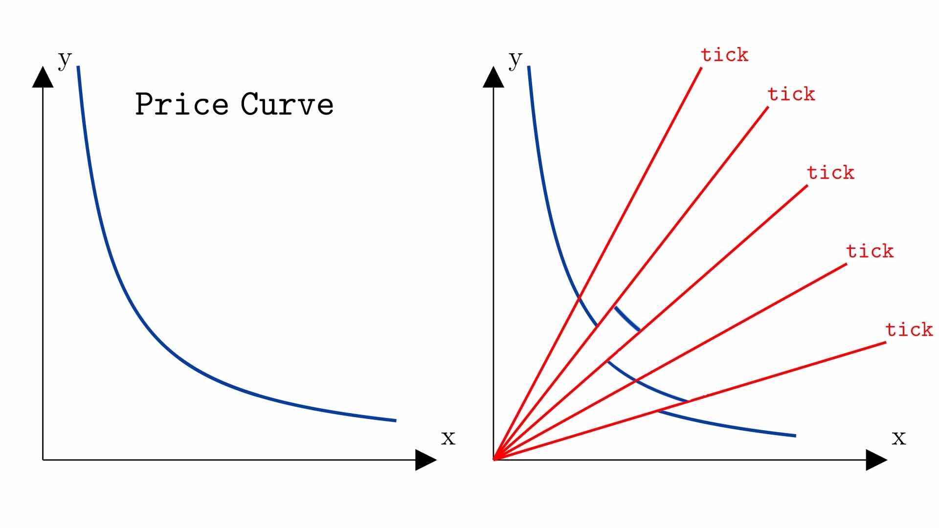
How these ticks are chosen and spaced is the subject of a later chapter.
Uniswap V3 Invariant
Uniswap V3 can be conceptualized as using the following invariant:
That invariant enables LPs to provide different liquidity between various ticks. Hence the values vary at different points in the curve.
The following interactive tool shows how changing for different segments changes that segment’s distance from the origin. Despite the curves not “touching each other,” the price can still move smoothly between sub curves (unless for a particular segment, in which case that segment is skipped). In practice, the segments are much smaller than shown in the tool below:
Piecewise formula is for illustration only
In practice, it is not gas-efficient to check the price against so many potential cases like we do in the formula above. Similarly, keeping track of so many values is expensive.
Therefore, Uniswap V3 accomplishes the piecewise formula above using an alternate mechanism which is so complex that it is the subject of about a half of this book. The mechanism will be revisited in later chapters.
However, if we visualize the Uniswap V3 curve, it looks like the curve shown above.
Exercise: Move the sliders in the image to all have the same value. Note that this produces a curve that is identical to a Uniswap V2 curve, except that the curve does not extend to infinity and 0.
How liquidity gets distributed in practice
It is possible that some values for different segments might be the same. For example, it might be the case that . It also might be the case that some of the values are zero if no liquidity was placed in that price range.
Each entirely depends on where LPs chose to add liquidity.
However, LPs will tend to place liquidity around where they expect trades to happen, because Uniswap V3 only awards LPs with swap fees if their liquidity is actually used (how this is accounted for is discussed in a later chapter).
In the screen recording below, we see the Uniswap V3 LP user interface for the ETH/USDC V3 pool on Base. The gray vertical line is the current price, and the two blue lines are the lower and upper predefined price where Uniswap V3 allows LPs to add liquidity. Note that the blue lines cannot be set to arbitrary locations, but only at predefined prices.
Here is a plot showing what a Uniswap V3 curve might look like for a pool of two stablecoins.
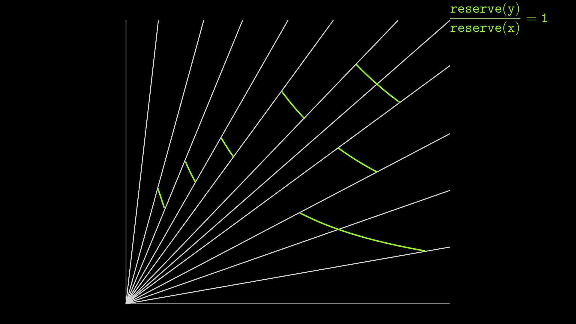
A price of 1:1, which we expect for a stablecoin pair, corresponds to the 45 degree ray where the ratio of reserves equals 1. Hence the liquidity ends up concentrated around center region where the ratio of reserves is 1 to 1 :
Below is a screenshot of how Uniswap V3 visualizes concentrated liquidity. In the USDC / USDT pool below, we see there is high liquidity around the price 1.000, which is where LPs expect the trades to occur:
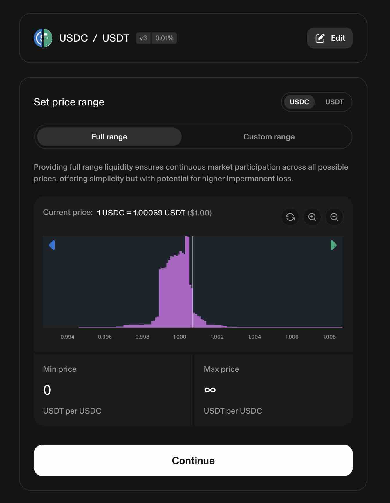
(The graphic above can be found by going to the USDC/USDT pool on mainnet, and then clicking “Add Liquidity”)
For a pool where token0 is more expensive than token1, the liquidity will tend to be more concentrated around that price:
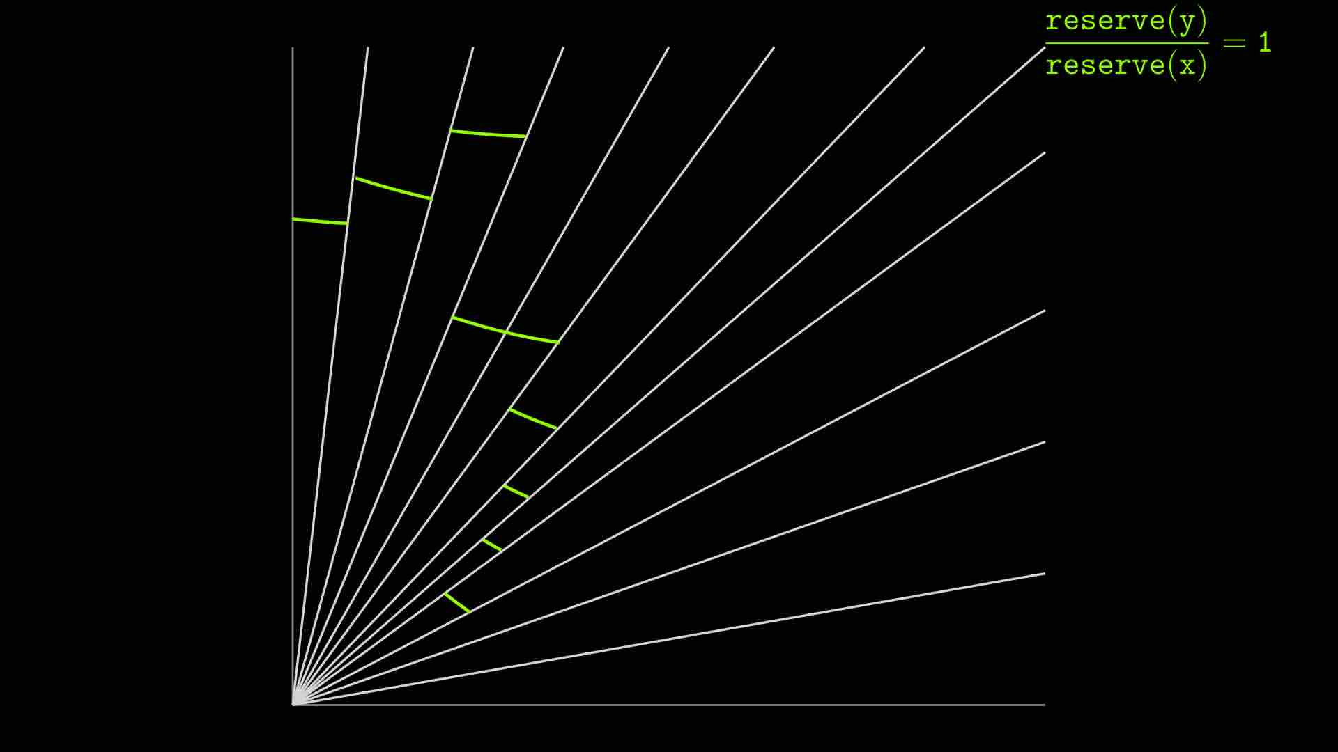
If the market price changes significantly, then liquidity providers will remove their liquidity and place it around the new price to capture the swap fees.
Crossing ticks causes no disruption
Even though the curve is discontinuous, a trader can still trade seamlessly between ticks. Once a tick is crossed, Uniswap V3 recalculates the amount of liquidity available for the rest of the trade as the following animation shows:
When the price crossed the tick, the reserves suddenly jumped up because the swap enters a region where the liquidity is higher, and hence the reserves are higher. This jump in reserves reflects the increased amount of reserves that LPs previously put in that price range.
Conclusion
Despite how intimidating the Uniswap V3 codebase may seem, the resulting mechanism is very simple at a high level.
Uniswap V3 has the same fundamental mechanisms as Uniswap V2:
- LPs can add and remove liquidity, although in V3 they have more choice about where to provide the liquidity.
- Swappers can exchange one token for another.
- Both protocols provide an oracle for tracking and retrieving previous prices.
The Uniswap V3 curve is a Uniswap V2 curve where the liquidity potentially changes at preset prices (ticks), depending on how the LPs placed their liquidity.
Such a design enables LPs to concentrate their liquidity around what they believe is the market price of the asset. With higher liquidity, traders will get a lower price impact, making that pool a more competitive choice for traders.