Real and virtual reserves in Uniswap v3

Uniswap v3 uses two types of reserves: real reserves and virtual reserves.

Real reserves represent the actual amount of tokens present in a segment.

Each segment has a pair of real reserves: the real reserves in token X, denoted by $x_r$, and the real reserves in token Y, denoted by $y_r$.The reserves for one of the tokens may be zero, but not for both — otherwise, there is no liquidity in the segment.

Virtual reserves represent the amount of tokens a segment would have if it were part of an infinite curve—in other words, if the segment extended to infinity, like Uniswap v2.

We will begin this chapter by studying real reserves in more detail, then move on to virtual reserves.

The real reserves

Let’s consider the illustration below, which shows a single segment. The current price is represented by the red ray. This segment has $x_r$ real reserves in token X and $y_r$ real reserves in token Y, as shown geometrically in the illustration.

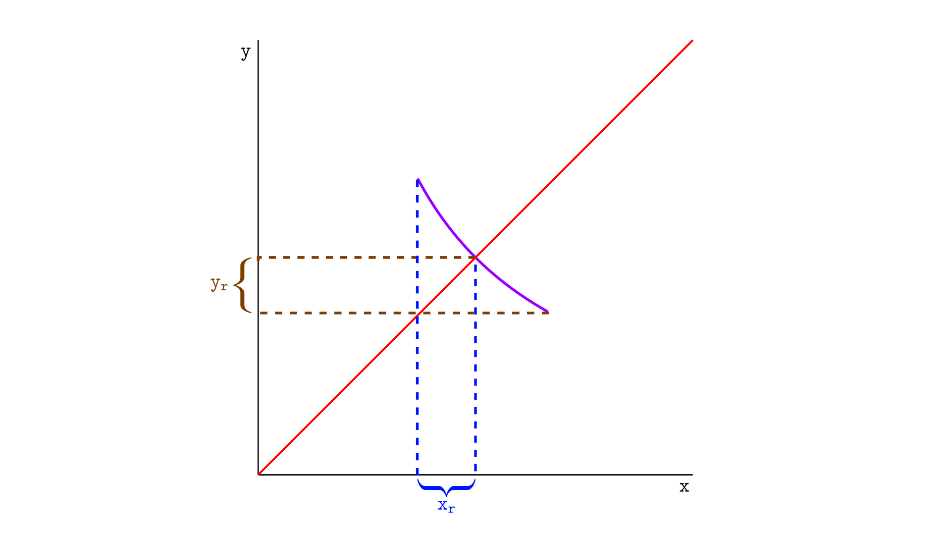
The real reserve of token X is the distance between the x-coordinate of the price and the x-coordinate of the upper tick. The same goes for token Y, but now it’s the distance in y to the lower tick.

The reason for this definition is that we are dealing with a curve segment. If the curve were infinite, the values $x_r$ and $y_r$ would be equal to $x$ and $y$, respectively.

One important difference between reserves in a segment—used in Uniswap v3—and in an infinite curve—used in Uniswap v2—is that, in a segment, a token can be completely depleted.

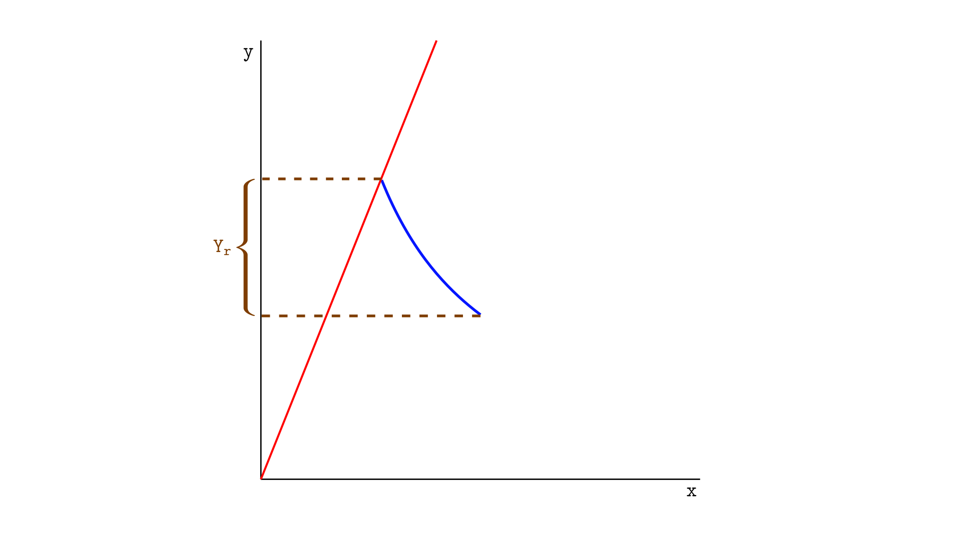
Imagine that, through a swap, the price moves to the position shown in the image below. In this case, all tokens X will be removed from the segment, and the real reserves will consist only of tokens Y.

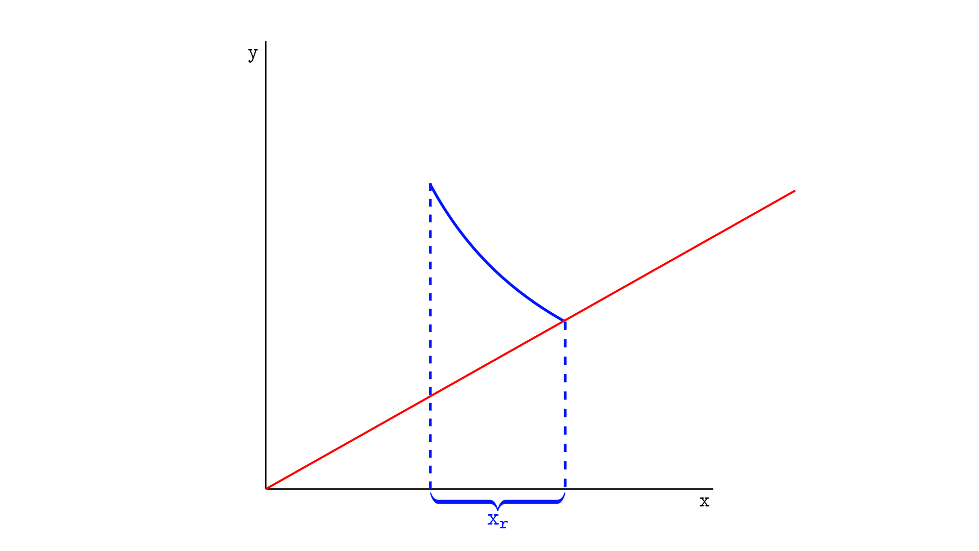
Another possibility is that the price moves all the way to the lower tick, as illustrated below. In this case, the segment’s real reserves will consist entirely of token X, and the segment will be completely depleted of token Y.

Such depletions are not possible in Uniswap v2 because the curve is infinite, so there is no “boundary” to be reached.

A pool in a real-world scenario is composed of more than one segment. Consider the scenario illustrated below: in this case, the price may fall below the blue segment, entering the violet segment.

The blue segment no longer has token Y to sell — its real reserves are only in token X — whereas the violet segment does. As long as the current price remains within the boundaries of a segment, the segment holds both tokens, and swaps can occur within it.

The amount of tokens X in the blue segment remain $x_r$ as long as the price continues lower than the lower tick.

As one can see, the real reserves of a segment depend on the current price. The rule is as follows:

1. If the current price is greater than or equal to the upper tick of the segment, the real reserves will be entirely in token Y.
2. If the current price is less than or equal to the lower tick of the segment, the real reserves will be entirely in token X.
3. If the current price is between the lower and upper ticks, there will be real reserves in both tokens X and Y.

Each segment has its real reserves

Real reserves exist for each segment—that is, each segment has a pair of values, $x_r$ and $y_r$, one of which can be zero but not both. If both are zero, there is no liquidity, and we can disregard the segment.

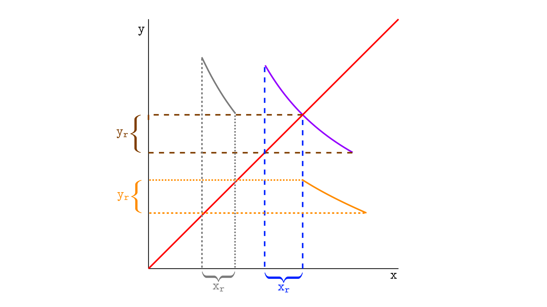
Consider the illustration below, which shows three segments—gray, purple, and orange (other possible segments are not shown). The current price is indicated by the red ray. Each segment has an amount for its real reserves.

• The gray segment has $x_r$ real reserves in token X and no real reserves in token Y.
• The purple segment has $x_r$ real reserves in token X and $y_r$ real reserves in token Y.
• The orange segment has $y_r$ real reserves in token Y and no real reserves in token X.

If the current price is outside a segment with liquidity, that segment necessarily contains only one asset. Any change in price that does not enter the segment in question will not affect the real reserves in that segment.

When the price moves within a segment, tokens X and Y are exchanged through swaps. Thus, each segment functions like Uniswap v2 when the price is within it but becomes inactive when the price is outside it.

But Unsiwap v2’s math works when the segment is actually an infinite curve. In order to treat each segment as if it were an infinite curve—and thus behave like Uniswap v2—we introduce the concept of virtual reserves.

Virtual reserves

Virtual reserves are the reserves a segment would have if it were part of an infinite curve rather than just a segment. To illustrate this, let’s draw a infinite curve, dashing the parts outside the segment.

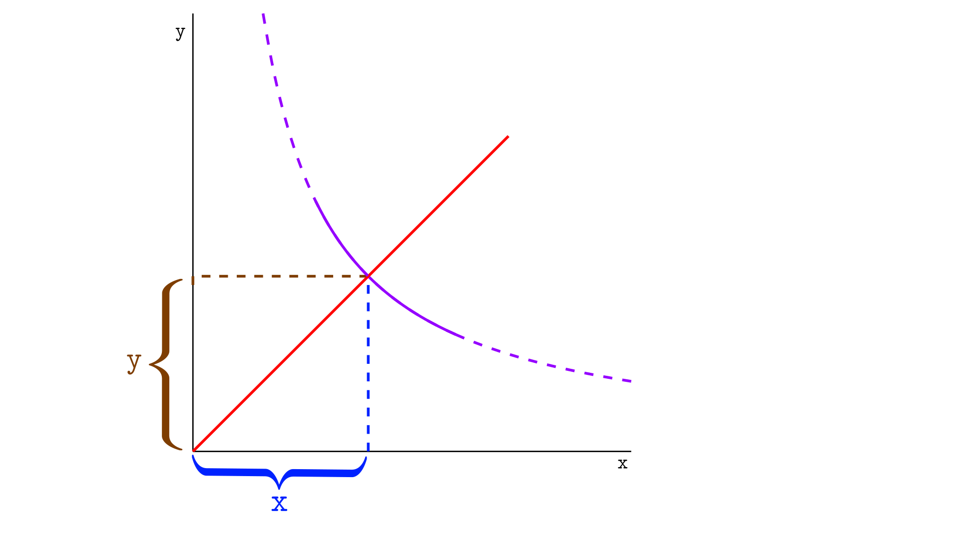
The virtual reserves are the reserves as if we were in Uniswap v2— in that case, they would be the reserves of the pool. The reserves are also the point $(x,y)$ where the current price touches the curve.

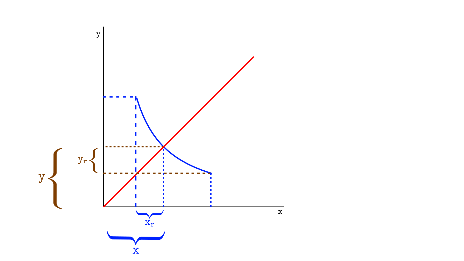
The illustration below shows both virtual $(x,y)$ and real reserves $(x_r, y_r)$ for the segment.

The animation below shows that, as the curve segment grows, the real reserves of the segment approach the virtual reserves. If the curve extends to infinity—as in Uniswap v2—the virtual and real reserves become the same.

Why don’t we need virtual and real reserves in Uniswap v2?

In Uniswap v2, since there is only a single, infinite price curve—and not several curve segments—real reserves and virtual reserves are the same. Thus, the coordinates $(x,y)$ represent both virtual and real reserves. We don’t need to distinguish between them and can simply refer to them as reserves.

Swaps in segments occur in the same way as in Uniswap v2

Even though virtual reserves do not represent an actual amount of tokens for a segment—or for the pool—they are important because, within a segment, we want to use the same math as Uniswap v2. In other words, we want each segment to behave as if we were on an infinite curve —which is exactly what virtual reserves provide. We can make this simplification as long as a trade does not cause the price to move outside the segment.

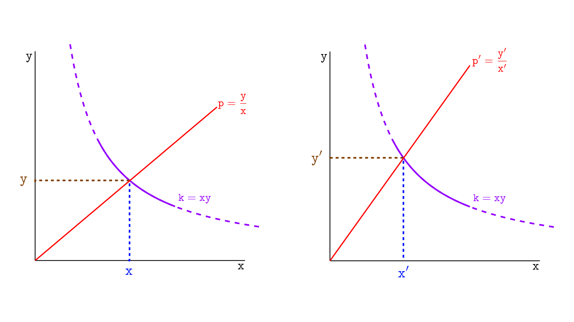
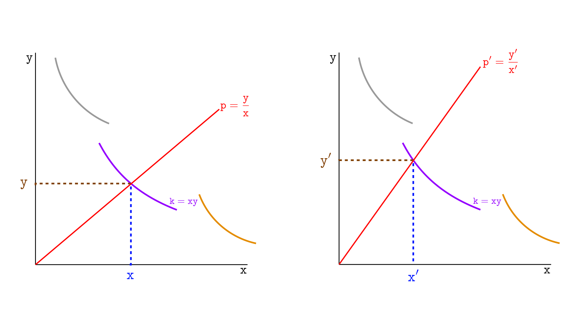
Consider the swap illustrated below, in Uniswap v2. At left, the pool contains $x$ tokens X and $y$ tokens Y, so the price is $y/x$ and liquidity is $xy$.

After a swap (on the right), the price becomes $y’/x’$; the reserves in token X change to $x’$, and the reserves in token Y change to $y’$. So, $(x-x’)$ tokens X leave the pool and $(y’-y)$ tokens Y enter the pool.

Now let’s consider the same swap, but this time in Uniswap v3, as illustrated below. We no longer have an infinite curve—just segments, like the three shown: gray, violet, and orange. Suppose the swap occurs in the violet segment, which has the same liquidity as the example above.

Note that everything happens the same way, as if the violet segment were an infinite curve! The price moves from $y/x$ to $y’/x’$; $(x-x’)$ tokens X leave the pool, and $(y-y’)$ tokens Y enter the pool.

Within a segment with liquidity $xy$, swaps occur exactly as if we were on an infinite curve with constant liquidity $xy$, as in Uniswap v2. The only two differences are:

1. When the price reaches the segment boundaries, swaps can no longer occur in that segment—they must occur in the next segment.
2. The $x$ and $y$ values of the segment do not represent the actual amount of tokens in that segment—they are the segment’s virtual reserves.

Other than that, we continue to use the same definitions as in Uniswap v2. The price of a token is defined by $p =y/x$, and liquidity follows the constant product formula $k=xy$.

The only difference is that we replace $k$ with $L^2$ and define liquidity as $L^2=xy$. The reason for this will become clear in a later section.

Price and liquidity in Uniswap v3

In Uniswap v3, we define price as the ratio between the virtual reserves,

$$ p = y/x $$

where price is always the price of token X.

Liquidity $L$ of a segment is defined by the formula

$$ L^2 = xy$$

An interactive tool for real and virtual reserves

Below is an interactive tool where you can see the real reserves $(x_r,y_r)$ and virtual reserves $(x,y)$ for a given segment. Slide the price to see how the reserves change as the price moves. You can also adjust the liquidity of the segments by changing k1–k4 below.

Calculating the real reserves of a segment

In the first sections of this chapter, we saw a visual representation of a segment’s real reserves. Now, we want a formula to calculate real reserves quantitatively.

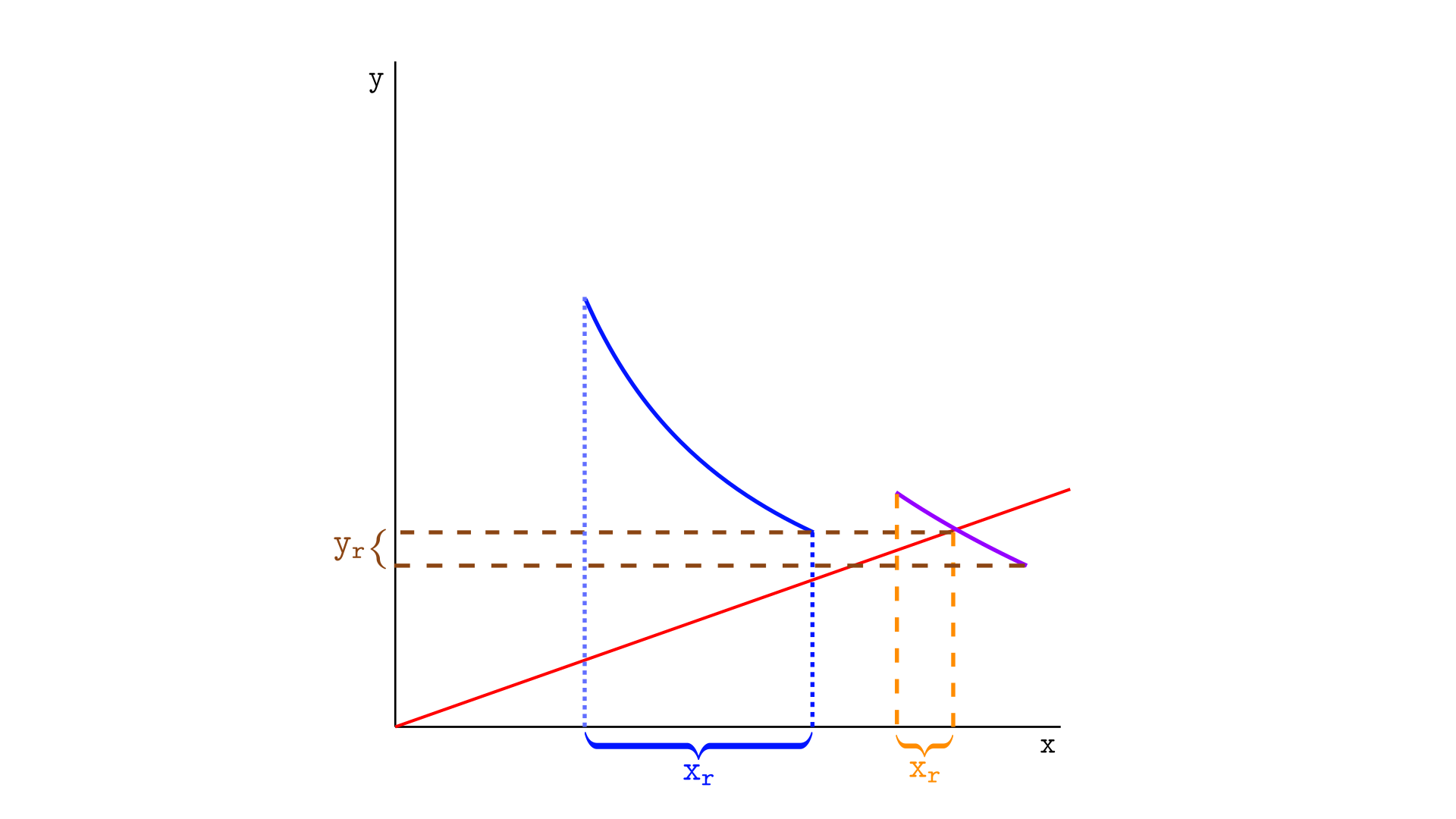
In Uniswap v2, reserves depend only on price and liquidity. In Uniswap v3, this cannot be the case. Let’s look at the illustration below. Both segments, on the left and on the right, have the same liquidity, and we are considering the same price, but clearly, the real reserves on the left are larger than those on the right.

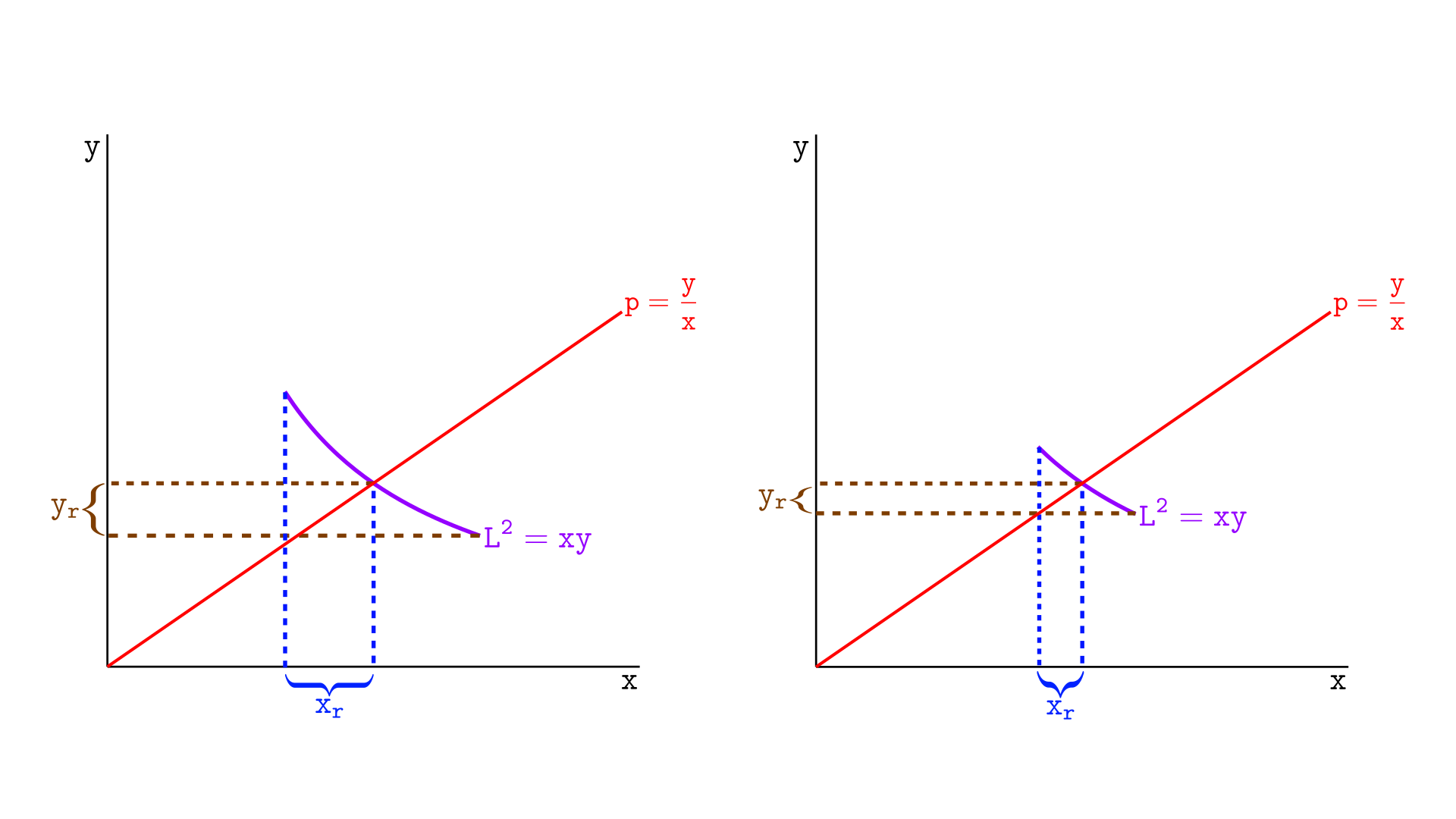
In Uniswap v3, a segment’s real reserves depend on the segment’s liquidity, the current price, and the segment’s boundaries—its upper and lower ticks. We will postpone deriving the formula for a segment’s real reserves until the next chapter.

Next, we will show how to calculate virtual reserves based on liquidity and price. This step is necessary before we can later explain how to calculate real reserves.

Deriving the virtual reserves from price and liquidity

We will now learn how to calculate the virtual reserves based on the current price and liquidity.

Deriving the virtual reserve $x$

We start with the definitions $L^2=xy$ and $p=y/x$, where $x$ and $y$ are the virtual reserves, $p$ is the price and $L$ the liquidity.

First, let’s divide $L^2$ by $p$ to derive $x$ in terms of $L$ and $p$:

$$ \begin{align*} \frac{L^2}{p} &= \frac{xy}{p} && \text{divide both sides of }L^2=xy\text{ by }p\\ \frac{L^2}{p} &= \frac{xy}{y/x}&& \text{substitute }p \text{ on the right hand side to } y/x \\ &= (x\bcancel{y}) \left(\frac{x}{\bcancel{y}}\right) &&\text{cancel }y\\ \frac{L^2}{p} &= x^2 &&\text{simplify}\\ \sqrt{\frac{L^2}{p}} &= \sqrt{x^2} &&\text{square root both sides}\\ \frac{L}{\sqrt{p}} &= x &&\text{simplify}\\ \end{align*}$$

Deriving the virtual reserve $y$

By multiplying $L^2$ by $p$, we can find the reserve $y$ as:

$$ \begin{align*} L^2 p &= (\underbrace{\bcancel{x}y}_{L^2}) (\underbrace{\frac{y}{\bcancel{x}}}_p) \\ L^2 p &= y^2 \\ L \sqrt{p} &= y && \text{square root on both sides} \end{align*}$$

The formulas for virtual reserves

We derived the two formulas we need: the virtual reserves calculated from $L$ and $\sqrt{p}$:

$$ \begin{align*} x &= \frac{L}{\sqrt{p}} \\ y &= L \sqrt{p} \end{align*}$$

Why do we use $L^2$ instead of $L$ when defining liquidity

If we had defined liquidity as $xy=L$ instead of $xy=L^2$, the above equations for $x$ and $y$ would have depended on $\sqrt{L}$ instead of $L.$ This can be seen in the derivation below, where we used $xy=L$ instead of $xy=L^2$.

$$ \begin{align*} \frac{L}{p} &= \frac{xy}{p} \\ \frac{L}{p} &= \frac{xy}{y/x}\\ \frac{L}{p}&= (x\bcancel{y}) \left(\frac{x}{\bcancel{y}}\right) \\ \frac{L}{p} &= x^2 \\ \sqrt{\frac{L}{p}} &= \sqrt{x^2} \\ \frac{\sqrt{L}}{\sqrt{p}} &= x \\ \end{align*}$$

Uniswap v3 uses $xy=L^2$ instead of $xy=L$ to avoid the costly operation of computing the square root on chain.

Motivation behind tracking the square root price instead of the price

Using $L^2$ allows us to avoid taking the square root of $L$ to compute $x$ and $y$, and it would be convenient if we could do the same for $p$. That is, it would be convenient if we could compute $x$ and $y$ from $L$ and $p$, rather than from $L$ and $\sqrt{p}$.

Unfortunately, this is not possible, since we don’t want to change how price is defined – we want to keep the same formula as v2. Thus, virtual reserves must be calculated using the formulas $x=L/\sqrt{p}$ and $y = L \sqrt{p}$.

This leaves us with two options: either track $p$ in the protocol and take its square root on-chain to calculate the reserves, or directly track the square root of $p$. The second option is much more gas-efficient.

Therefore, instead of tracking the price $p$, the protocol tracks the value $\sqrt{p}$ as the variable sqrtPriceX96, thus avoiding the need to compute the square root of price.

Summary

• Uniswap v3 has two types of reserves: virtual reserves and real reserves.
• Real reserves are defined per segment and indicate the amount of tokens contained in that segment. A segment can contain real reserves of tokens X, tokens Y, or both.
• The amount of tokens in a segment depends on the current price. If the current price is greater than or equal to the upper tick, there will be real reserves only in tokens Y. If it is less than or equal to the lower tick, there will be real reserves only in tokens X. If it is between the upper and lower ticks, there will be real reserves in both tokens.
• Virtual reserves are the amount of tokens a segment would have if it were an infinite curve – just like in Uniswap v2. Using virtual reserves, we can use the same math from Uniswap v2 on each segment of Uniswap v3.
• Uniswap v3 uses the formula $L^2 = xy$ instead of $L=xy$ to avoid having to calculate the square root of $L$ on-chain.
• The virtual reserves as a function of $L$ and $\sqrt{p}$ are given by $x=L/\sqrt{p}$ and $y=L\sqrt{p}$.