We’ll start this chapter on an unusual note — the NTT algorithm is quite simple and can be implemented in less than 20 lines of code. However, the key idea that makes it work, oddly enough, does not have a formal mathematical name. So we are going to take the liberty to give what we believe to be the core theorem behind the algorithm a (subjectively) catchy name:
The Image Preservation Theorem for Multivalued Functions
To explain the Image Preservation Theorem, we’ll go over one last (very simple) concept about roots of unity, then introduce the theorem.
-th roots of nested square roots
The literal definition for “k-th root of unity” is that the root of unity satisfies . Stated another way:
Therefore, it should be no surprise that if is the primitive 4-th root of unity then
Now let’s do the same operation if is the primitive 8-th root of unity. The result would be
and the 8-th root of 1 generates all the 8-th roots of unity:
These observations are simply a matter of definition. Of course, we do not want to directly compute the square root of 1. It’s much easier to first find the primitive -th root of unity first, then generate the set of answers for . For example:
import galois
Fq = 17
k = 8
assert (Fq - 1) % k == 0, "no such subgroup"
GF = galois.GF(Fq)
pr = GF.primitive_root_of_unity(k)
roots = []
for i in range(0,k):
roots.append(pr**i)
print(roots)
We can also observe that:
and so on. As noted above, directly computing the is not efficient. Instead, we consider the following diagram, where each arrow down is a square root of the number above it:
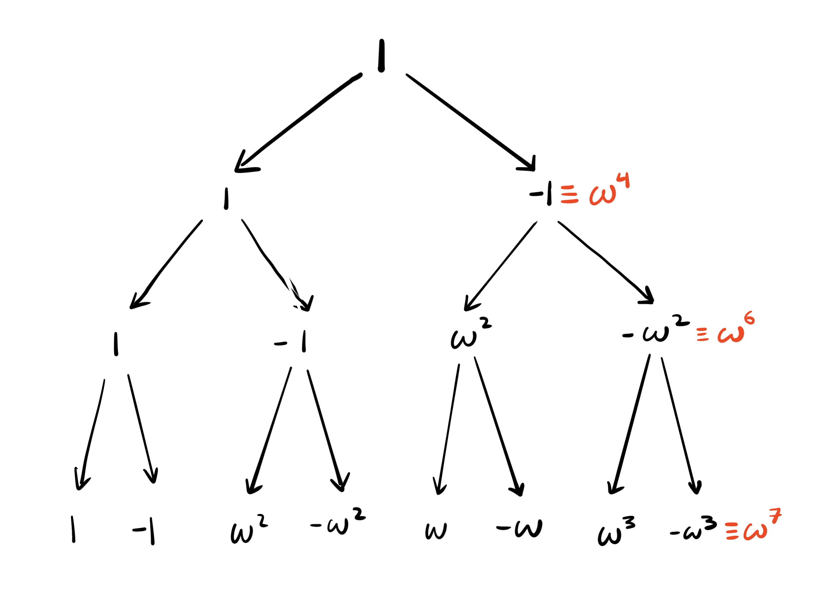
We can compute the 8-th roots of unity by starting with 1 and repeatedly taking square roots.
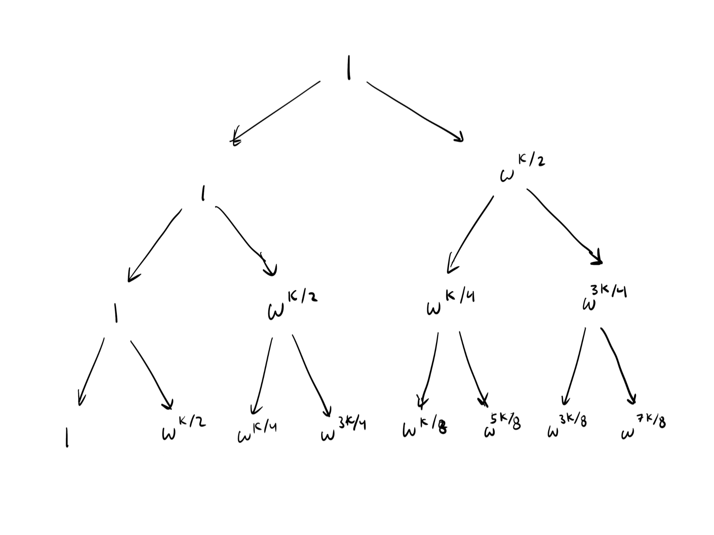
For arbitrary , the diagram is as follows.
Here is a walkthrough of the square root computations:
The square root of 1 is . is congruent to -1
Recall from the previous chapter that the square root of is and (assuming is even).
Thus, the square root of is .
Also recall that the additive inverse of is .
So to compute without the negative sign, we compute . So the square root of is .
The square root of is . Again, to get rid of the negative sign, we compute
Why the square root of is left as an exercise for the reader.
The height of the tree is
Computing the -th roots of unity by repeatedly taking the square roots of 1 creates a “tree” that is in height.
Conceptualizing intermediate states of the tree
The set
is mathematically equivalent to the 8-th roots of unity. The set is also equivalent:
Which is also equivalent to:
In other words:
Quick aside — multivalued functions and images
Admittedly, the observations we made above are trivial extensions of the definition of -th roots. The more interesting implications of these observations will be shown in the following section. However, it will be helpful to introduce some mathematical terminology first:
Image of a function — if we have a set of points that we evaluate a function on, then the set of evaluations is the image. For example, if the function is and the domain we evaluate on is then the image will be . The term range of a function means the set of values a function could output. In our context, the image of the function refers to the actual set of outputs for a given set of inputs.
Multivalued function — a function that may return more than one evaluation for a single point in the domain. For example, evaluated on 0 returns 0, but evaluated on 1 returns .
Note: The multivalued function has an image larger than its domain.
With these definitions in mind, the reader should understand the following statements:
“The image of on the domain is ”
“The image of the multivalued function on the domain is ”
Now we get to a more interesting set of observations.
The image of evaluated on is the same as evaluated on (k = 8)
This claim is a simple rephrasing of the concepts shown above, so we won’t elaborate further. The interesting part is how we can generalize this to other functions.
The nuance here is that is a multivalued function that returns eight elements.
The image of evaluated on the 4-th roots of unity is the same as the multivalued function evaluated on (k = 4)
Remember, , so . This is the same image as evaluating on each root of unity one-by-one. Since
Exercise for the reader: Let . What is the image of on the 4-th roots of unity? What is the image of the multivalued function on the domain ?
In the following chapters, we will show how to handle more complex cases like , but for now, we show how to actually compute multivalued functions for the simple cases we showed here. But first, let’s give a formal definition to the observation we’ve made so far about image equivalence.
The image of evaluated on the 4-th roots of unity is the same as the multivalued function evaluated on the second roots of unity (k = 4)
This example is very similar to the above, except that we don’t “target” the domain but rather .
We have that
This is the same image as evaluating on
In summary, if we “shrink” the domain by a factor of and replace every in with to create a new multivalued function , the images of and are identical.
We’ll now formally define the concept we’ve been illustrating
The core theorem of NTT: Image Preservation Theorem for Multivalued Functions
Let be the primitive -th root of unity and be the -th roots of unity defined in .
Let be a power of 2.
Let be a polynomial in . Let be a power of 2 less than or equal to .
Let be a multivalued function created by replacing every in with .
Let the domain be . Note that if then .
The image of on exactly equals the image of on .
It is of utmost importance that the reader understand the theorem above, as it is the key concept that the Number Theoretic Transform relies on!
Here are some examples to enforce the concept:
- The image of on the 4-th roots of unity is equal to the image of on the second roots of unity (as shown in the previous section).
- The image of on 16th roots of unity is equal to image of on 8th roots of unity
- The image of on k-th roots of unity is equal to image of on k/2-th roots of unity
- The image of on k/2-th roots of unity is equal to image of on k/4-th roots of unity
The following section shows examples where is slightly more complex.
Image Preservation Theorem Examples for
Let and the domain be the 4-th roots of unity .
Let be the multivalued function and the domain be or equivalently .
Let be the multivalued function and the domain be
The images of , , and are identical:
Connection to NTT
Remember, the goal of NTT is to evaluate on the -th roots of unity in time. In other words, we want to compute the image of on the -th roots of unity.
You can probably guess where this is going.
Computing the image of on the -th roots of unity is equivalent to computing the image of a new function defined such that for each in , evaluated on .
However, this leaves an open question:
Expanding into doesn’t directly lead to a speedup. Algorithmically, expanding a into the -th roots of unity is the same as evaluating on the points. How does this alternate way of evaluating help us?
In the next chapter, we will demonstrate how to evaluate multi-valued functions using square root expansion and explain how this approach can prevent redundant computation.