Multiplication of Polynomials in Point Form

Polynomial multiplication is widely used in zero-knowledge proofs and mathematical cryptography. But the brute force or traditional approach for multiplying polynomials runs in $\mathcal{O}(n^2)$, which is fine for small inputs but becomes quite expensive as the degree of the polynomial increases. This article takes a detailed look at polynomial multiplication in order to explore ways of making it faster.

• We begin with a review of the schoolbook/traditional polynomial arithmetic
• Followed by a study of different forms of representation of polynomials
• We examine and compare polynomial arithmetic in these different forms
• Finally, we look at how these forms can potentially speed up polynomial multiplication – and how they form the grounds for an algorithm called Number Theoretic Transform (NTT)

Polynomial Multiplication – Traditional approach

Consider two polynomials $p_1(x)$ and $p_2(x)$ of degree $n$ each:

$$ p_1(x) = a_0 + a_1x + a_2x^2 + \dots + a_nx^n \\p_2(x) = b_0 + b_1x + b_2x^2 + \dots + b_nx^n$$

Multiplying these two polynomials using the simple way of distribution of multiplication over addition takes $\mathcal{O}(n^2)$. Here, each term of $p_1(x)$ is multiplied with each term of $p_2(x)$:

$$ \begin{aligned} p_1(x) \cdot p_2(x) &= p_1(x)\cdot (b_0 + b_1x + \dots + b_nx^n) \\ &= (a_0 + a_1x + \dots + a_nx^n)\cdot (b_0 + b_1x + \dots + b_nx^n) \\ &= a_0\cdot (b_0 + b_1x + \dots + b_nx^n) \\ &+ a_1x\cdot (b_0 + b_1x + \dots + b_nx^n) \\ & \vdots\\ &+ a_nx^n\cdot (b_0 + b_1x + \dots + b_nx^n) \end{aligned}$$

For example, let $p_1(x) = 1 + 2x$, and $p_2(x) = 3 + 4x$.

Then,

When programmed, this is implemented in the form of nested loops.

# Let A be array representing the coefficients of p1(x)
A = [a0, a1, ..., an]
# Let B be array representing the coefficients of p2(x)
B = [b0, b1, ..., bn]
# Let C be the array storing coefficients of p1(x).p2(x)

function multiply_polynomials(A, B):
    n = len(A)
    m = len(B)
    C = array of zeros of length (n + m - 1)

    for i from 0 to n - 1:
        for j from 0 to m - 1:
            C[i + j] += A[i] * B[j]
    return C

You would get the result as:

$$ \begin{array}{c|cc} \times & 3 & 4x \\ \hline 1 & 3 & 4x \\ 2x & 6x & 8x^2 \end{array}$$

For each $n$ iterations of the outer loop, the inner loop executes n times (assuming equal degree $m=n$), thus giving n times n, i.e. runtime of $\mathcal{O}(n^2)$.

We now want to see if we can optimize this and do better. Or simply, is there a way to make polynomial multiplication faster?

Ways to represent a Polynomial

There are two ways in which we can represent a polynomial: coefficient form and point form.

Coefficient Form

Polynomials are usually expressed in what is called the monomial basis, or the coefficient form, meaning it’s written as a linear combination of powers of the variable.

For instance, a polynomial of degree $n$, when expressed as

$$ p(x) = a_0 + a_1 x + a_2 x^2 + \dots + a_n x^n$$

is expressed in the monomial basis, since it is using $[1, x, x^2, …, x^n]$ as the basis for its coefficients, which are $a_0, a_1, a_2, .., a_x.$

In this representation, the coefficients of $p(x)$ can be written as a vector or an array, like $[a_0, a_1, …, a_n]$, where the first element corresponds to the constant term or coefficient of $x^0$, while the last element corresponds to the coefficient of $x^n$.

You should note that the earlier method of distributive multiplication we looked at (runtime $\mathcal{O}(n^2)$) was applied over the coefficient form of polynomials.

Point (or Value) Form

The point (or value) form representation is based on the fact that every polynomial of degree $n$ can be represented by a set of $n+1$ distinct points that lie on it.

For example, consider a quadratic polynomial (degree $2$):

$$ 2x^2-3x+1$$

Now take any $3$ (because $n=2$) lying on this curve, say $(0,1)$, $(1,0)$ and $(2,3)$. We can say that these $3$ points represent the given polynomial. Alternatively, if we are just given these points, it is possible to recover the polynomial $2x^2 -3x+1$ from that information. Why does this work? Or how are we able to equivalently represent a degree $n$ polynomial with $n+1$ points?

This is because:

For every set of $n+1$ distinct points, there exists a unique lowest degree polynomial of degree at most $n$ that passes through all of them.

This lowest degree polynomial is called the Lagrange Polynomial.

For example, given two points $(1, 2)$ and $(3, 4)$, there exists a unique polynomial of degree $1$ (a line) passing through these points:

$$ p(x) = 1 + x$$

Similarly, given three points $(0, 1)$, $(1, 4)$, and $(2, 9)$, the Lagrange polynomial of degree $2$ passing through these points is:

$$ p(x) = 1 +2x+ x^2 \\ 1 + 2(0) + (0)^2 = 1 \\ 1 + 2(1) + (1)^2 = 4 \\ 1 + 2(2) + (2)^2 = 9$$

How this special polynomial is calculated given a set of points is something that is discussed in this article on Lagrange interpolation.

Uniqueness of the Lagrange Polynomial

You must note that for a set of points, there are multiple polynomials of a given degree that pass through all of them. But only the lowest degree polynomial is unique.

For instance, in the above example of points $(1, 2)$ and $(3, 4)$, there exist many polynomials passing through these two points: $x^2 -3x +4$ and $2x^2 -7x +7$ are two of many polynomials of degree $2$ (quadratic) that pass through these two points.

Similarly, if you consider degree $3$, two example polynomials passing through points $(1,2)$ and $(3,4)$ are $x^3 -5x^2 +8x-2$ and $-x^{3}+4x^{2}-2x+1$.

But for the lowest degree, here $1$, there exists only one polynomial of the lowest degree, and that is $p(x) = 1 + x$. It is unique, and there is no other polynomial of degree $1$ that can pass through these two given points.

How is this lowest degree determined?

For every set of $n+1$ distinct points, there is a unique polynomial of degree at most $n$ that passes through them. The degree of the unique polynomial is less than $n$ if some of the points are collinear or lie on a lower degree polynomial. Therefore, we use the term “at most $n$” to cover the case where the degree is exactly $n$, as well as cases where the degree is lower.

For example, given the points $(1,2),(2,4),$ and $(3,6)$, the polynomial of lowest degree passing through them is $y=2x$. This is because the points are collinear, i.e. they lie on a line. One can check that the slope between any pair of them is the same:

$$ \frac{4-2}{2-1} = \frac{6-4}{3-2} = 2$$

Therefore, the lowest degree is $1$, and $y=2x$ is the unique Lagrange polynomial.

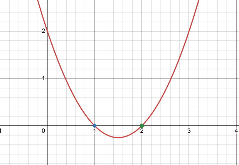
Similarly, Given five points, $(-2,1), (-1,0), (0,1), (1,4), (2,9)$, we find that all of them lie on a parabola with the equation

$$ y = x^2 + 2x + 1 $$

This is a case where all the given points lie on a lower degree polynomial, here degree $2$, and thus the Lagrange polynomial has degree $2$, which is less than $n$ (Here, $n=4$).

Refer to the Appendix at the end for proof of uniqueness of the lowest degree polynomial.

Conversion Between Coefficient Form and Point Form

Since coefficient form and point form are equivalent, we can readily convert between them as we show now.

Interpolation (Point Form → Coefficient Form)

The conversion from point form to coefficient form, called interpolation, is calculating the polynomial of lowest degree which passes through all the given points. One of the most well-known methods it is done is using Lagrange Interpolation, that we mentioned previously. If you are unfamiliar with it, you may go through this article.

In short, given a set of $(n+1)$ distinct points

$$ \{(x_0, y_0), (x_1, y_1), \dots, (x_n, y_n)\}$$

we can find the unique lowest degree polynomial $p(x)$ of degree at most $n$ using the formula for Lagrange interpolation, such that:

$$ p(x_i) = y_i \quad \text{for all } i = 0, 1, \dots, n $$

You should keep in mind that the runtime of Lagrange interpolation is $\mathcal{O}(n^2)$.

Evaluation (Coefficient Form → Point Form)

The conversion from coefficient form to point form, called evaluation, is evaluating the polynomial at values of $x$ to obtain the corresponding values of $y$, and thus a set of $(x_i, y_i)$ points, which represent the polynomial. One common way this can be done is by using Horner’s rule (to be discussed in detail in a future article).

In short, given coefficients $[a_0, a_1, \dots, a_n]$ of a polynomial $p(x)$ and a value $x_i$, Horner’s Method evaluates $p(x_i)$ as follows:

$$ p(x_i) = a_0 + x_i(a_1 + x_i(a_2 + \dots + x_i a_n) \dots)$$

This method factors out common powers of $x$, one at a time until all the terms are processed. Let us look at an example to understand it better.

Given the polynomial $p(x) = 2 + 3x + 5x^2 + x^3$ and a value $x = 2$, we will review how Horner’s rule evaluates $p(2)$.

We can rewrite $p(x)$ as follows (as shown in the generalized expression above):

$$ p(x) = 2 + x(3 + x(5 + x(1)))$$

Substituting $x = 2$:

Observe how the steps involve alternating multiplications and additions. Steps 1, 3 and 5 of the above calculation are multiplications, while steps 2, 4 and 6 are additions. In total, there are $n$ multiplications and $n$ additions (here $n=3$), giving a total runtime of $\mathcal{O}(n)$. This is how Horner’s rule evaluates a polynomial of degree $n$ at a given value of $x$ in $\mathcal{O}(n).$

Therefore, evaluating the polynomial at $n+1$ distinct $x$-values – converting from coefficient to point form using this rule – takes $n$ times $n+1$, i.e. $\mathcal{O}(n^2)$.

Coefficient form VS Point form

We said that coefficient form and point form of a polynomial are equivalent, and one can be converted to the other. That is, there is no difference in the final results of addition and multiplication when done in either form. Let us examine this, with an example of addition first.

Addition in coefficient form

Consider two polynomials given in coefficient form,

$$ p_1(x) = 1 + 2x + 3x^2 \\p_2(x) = 4 + 0x + 1x^2 $$

Or their respective arrays of coefficients:

$$ p_1: [1,\ 2,\ 3] \\p_2: [4,\ 0,\ 1]$$

Now, adding the two polynomials is simply adding the two arrays element-wise, and the resultant coefficient array represents the final polynomial. Let’s verify this:

$$ p_{\text{sum}}(x) = (1+4) + (2+0)x + (3+1)x^2 = 5 + 2x + 4x^2 $$

Or simply, $[(1+4), (2+0),(3+1)] = [5,\ 2,\ 4]$

For two polynomials of degree $n$, we perform $n+1$ additions to get the sum’s representation. Therefore, the runtime of addition in coefficient form is $\mathcal{O}(n)$.

Addition in point form

Consider the same two polynomials,

$$ p_1(x) = 1 + 2x + 3x^2 \\p_2(x) = 4 + 0x + 1x^2 $$

First, we need to convert them from coefficient form to point form. Since the degree of both polynomials is $2$, the degree of their sum will be at most $2$ as well. Therefore, we need three points to represent the sum (degree plus one: $n + 1$), which requires $3$ evaluations each of $p_1(x)$ and $p_2(x)$.

Let us evaluate $p_1(x)$ and $p_2(x)$ at $x = 0, 1, 2$ to get our points.

Note: We are just choosing $x=0,1,2$ for simplicity. You could pick any other $3$ points for evaluation.

• $p_1(0) = 1, \quad p_1(1)= 6, \quad p_1(2)=17$
• $p_2(0) = 4, \quad p_2(1)= 5, \quad p_2(2)=8$

Now, adding the two polynomials requires adding the corresponding evaluations element-wise, that is:

• $p_{\text{sum}}(0) = (1+4) =5$
• $p_{\text{sum}}(1) = (6+5) =11$
• $p_{\text{sum}}(2) = (17+8) =25$

These three points $(0, 5), (1, 11)$ and $(2, 25)$ give us the point representation of the sum. Let us verify whether they satisfy the polynomial we calculated earlier:

$$ p_{\text{sum}}(x) = 5 + 2x + 4x^2$$

• $p_{\text{sum}}(0) = 5$
• $p_{\text{sum}}(1) = 5 + 2 + 4 = 11$
• $p_{\text{sum}}(2) = 5 + 4 + 16 = 25$

Therefore, you see that addition in both forms gives the same result, or the same polynomial, just represented in different ways.

In point form addition, for two polynomials of degree $n$, there are $n+1$ points representing each of them, and thus $n+1$ element-wise additions that we perform to get the sum’s representative points. Therefore, the runtime of addition in point form is $\mathcal{O}(n)$.

Now, let us also look at multiplication closely.

Multiplication in coefficient form

Consider two polynomials given in coefficient form:

$$ p_1(x) = 1 + 2x\\p_2(x) = 3 + 4x$$

Or their respective coefficient arrays: $p_1 = [1,\ 2]$ and $p_2 = [3,\ 4]$

Multiplying them using the distributive way discussed earlier gives:

$$ \begin{aligned} p_{\text{prod}}(x) &= (1)(3+4x) + (2x)(3 + 4x) \\ &= 3 + 4x + 6x + 8x^2 \\&= 3 + 10x + 8x^2 \end{aligned} $$

The resulting polynomial is $p_{\text{prod}}(x) = 3 + 10x + 8x^2$, represented by the coefficient array $[3,\ 10,\ 8]$. The distributive method of coefficient form multiplication takes $\mathcal{O}(n^2)$, as we saw at the start of this article.

Multiplication in point form

We now consider the same polynomials and convert them to their point forms.

$$ p_1(x) = 1 + 2x\\p_2(x) = 3 + 4x $$

Since both polynomials have degree $1$, their product will have a degree of at most $2$, meaning we need $3$ points to represent it, which requires 3 evaluations of each of $p_1(x)$ and $p_2(x)$.

So, let’s evaluate $p_1(x)$ and $p_2(x)$ at $x = 0, 1, 2$.

• $p_1(0) = 1,\quad p_1(1) = 3,\quad p_1(2) = 5$
• $p_2(0) = 3,\quad p_2(1) = 7,\quad p_2(2) = 11$

Now, to get the points that represent their product, we multiply the evaluations element-wise:

• $p_{\text{prod}}(0) = 1 \cdot 3 = 3$
• $p_{\text{prod}}(1) = 3 \cdot 7 = 21$
• $p_{\text{prod}}(2) = 5 \cdot 11 = 55$

So the three points $(0, 3), (1, 21)$ and $(2, 55)$ give us the point representation of the resultant product.

Let’s verify if they satisfy the polynomial product we got earlier:

$$ p_{\text{prod}}(x) = 3 + 10x + 8x^2 $$

• $p_{\text{prod}}(0) = 3$
• $p_{\text{prod}}(1) = 3 + 10 + 8 = 21$
• $p_{\text{prod}}(2) = 3 + 20 + 32 = 55$

Therefore, you can see that multiplication in both forms gives the same polynomial, just represented in different ways.

In summary, for two polynomials $p_1(x)$ and $p_2(x)$ of degree $n$, their product will have a degree of at most $2n$, meaning we need $2n+1$ points to represent it. Thus, we perform $2n+1$ evaluations for each polynomial at common values of $x$ to convert them into point form:

$$ p_1(x_0), p_1(x_1), p_1(x_2), \dots p_1(x_{2n})\\p_2(x_0), p_2(x_1), p_2(x_2), \dots p_2(x_{2n})$$

We then perform point form multiplication by multiplying these two sets element-wise, which takes $2n+1$ multiplications, i.e., runtime of $\mathcal{O}(n)$.

$$ p_1(x_0) \cdot p_2(x_0), \; p_1(x_1) \cdot p_2(x_1), \dots, \; p_1(x_{2n}) \cdot p_2(x_{2n}) $$

This gives us the $2n+1$ points which represent the product $p_1(x).p_2(x)$:

$$ \{(x_0,p_1(x_0) \cdot p_2(x_0)), \; (x_1, p_1(x_1) \cdot p_2(x_1)), \dots, \; (x_{2n}, p_1(x_{2n}) \cdot p_2(x_{2n}))\} $$

The amazing thing to note here is that, while addition in both coefficient and point form takes the same time $\mathcal{O}(n)$, multiplication in point form is significantly faster than in coefficient form. In point form, we perform $2n+1$ element-wise multiplications, giving a runtime of $\mathcal{O}(n)$, which is way better than the $\mathcal{O}(n^2)$ required for coefficient form multiplication!

However, there is still an issue- we haven’t considered the overhead of converting to the point form and vice versa.

So, lets look at the complete process of multiplication in point form, which involves three steps:

1. Conversion of coefficient to point form We evaluate the two polynomials of degree $n$, to be multiplied, at $(2n+1)$ values of $x$, to get a set of $(2n+1)$ evaluations each. This takes $\mathcal{O}(n^2)$ using Horner’s Method.
2. Element-wise multiplication in point form representation We multiply these two sets element-wise to get $(2n+1)$ evaluations that gives the point form representation of their product. This takes $\mathcal{O}(n)$.
3. Conversion of point to coefficient form We calculate the unique lowest degree polynomial (coefficient form) that passes through all the resultant $(2n+1)$ points. This takes $\mathcal{O}(n^2)$ using Lagrange interpolation.

Therefore, the overall runtime for the steps above is:

$$ \mathcal{O}(n^2) + \mathcal{O}(n) + \mathcal{O}(n^2) \approx \mathcal{O}(n^2)$$

which is no better than where we started from. Thus, we need to explore whether any optimizations can make this process faster.

Optimizing conversion

The key point to keep in mind is that multiplication in coefficient form takes $\mathcal{O}(n^2)$, whereas multiplication in point form (element-wise) takes $\mathcal{O}(n)$. Therefore, if we can find a way to convert coefficient form to point form and vice versa (steps 1 and 3 mentioned above) faster than $\mathcal{O}(n^2)$, we can optimize multiplication to run in sub-quadratic time.

It is important to note that we cannot optimize polynomial addition, because addition in both coefficient form and point form runs in $\mathcal{O}(n)$ each.

So now let us brainstorm a few ways we might make the conversion from coefficient to point form faster.

What if we knew a point whose evaluation could give us the values of several related points, saving us from repeated calculations?

For example, if we had a polynomial with a symmetric graph, evaluating one point would tell us the evaluation for its corresponding symmetric point as well.

Consider the polynomial $p(x)= x^2$. Observe how,

$$ p(-2) = 4\space\space\space \text{and} \space\space\space p(2) =4$$

Or, more simply, observe how for all $x_i$,

$$ p(-x_i)=p(x_i)$$

This is not just true for $p(x)=x^2$, but generalizes to all polynomials that contain only even powered coefficients, which are also called as even polynomials.

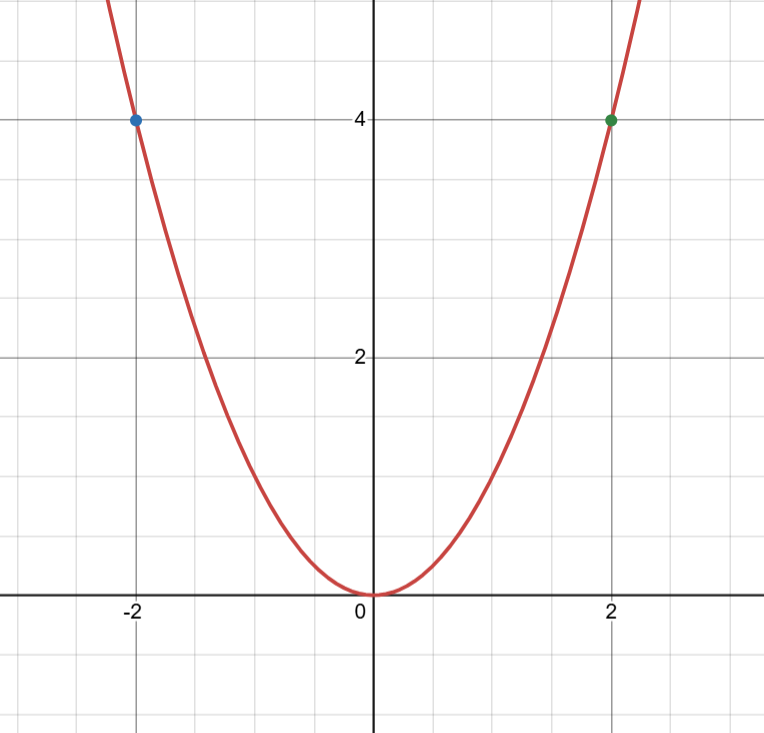
For example, consider the even polynomial (containing only terms with even powers of $x$:

$$ q(x) =x^{10}+3x^{8}-2x^{6}+3x^{4}-2x^{2}-x^{0} $$

In the graph above, it is easy to observe that

$$ q(x) =q(-x)$$

Visually speaking, the graphs of even polynomials are mirrored about the $y$-axis, and they evaluate to the same $y$ for both positive and negative values of any given $x$.

What about odd polynomials that contain only odd powered coefficients? Consider $p(x) = x^3$. Observe how

$$ p(-2) = -8 =-p(2)$$

In the graph above, observe how, for all $x_i$,

$$ p(-x_i) = -p(x_i)$$

Again, this is not just true for $p(x)=x^3$, but generalizes to all odd polynomials, i.e. polynomials containing only terms with odd powers of $x$. For example, consider the polynomial

$$ q(x)=-x^{7}+3x^{5}+x^{3}-x$$

In the graph above, observe that

$$ q(x) = -q(-x)$$

Visually, the graphs of all odd polynomials are symmetric about the origin, which makes the above equality true for all of them.

Now you can see that after evaluating certain points, we can get the evaluation at other points without any extra calculation. For instance, in the examples above, for even and odd polynomials, knowing the evaluation for $p(x)$ also gives us the evaluation for $p(-x)$.

We can exploit this fact to make polynomial multiplication faster, which is exactly what a beautiful algorithm called the Number Theoretic Transform (NTT) allows us to do. NTT enables evaluation and interpolation in $\mathcal{O}(n \log n)$ by recursively using properties of symmetries of certain points, thereby making the conversion sub-quadratic.

But since NTT operates over a finite field, there are no negative values of $x$ we can work with. This is where the concepts of multiplicative subgroups, cyclicity and roots of unity come into the picture. These concepts will allow us to exploit the symmetries present in finite fields to perform polynomial multiplication more efficiently. We’ll explore how NTT works in detail in upcoming articles.

Appendix

Uniqueness of lowest degree polynomial proof

We show that if there are two polynomials $p(x)$ and $q(x)$ of equal degree which interpolate a set of points, then a polynomial $r(x)$ must exist such that $r(x) = p(x)-q(x)$.

We will then show that the only possible solution for $r(x)$ is $r(x) = 0$, otherwise we end up with a polynomial that has more roots than its degree, which we show is impossible. Let us look at these steps in detail now.

Let us assume that the lowest degree Lagrange polynomial is not unique. Then there are at least two distinct polynomials of lowest degree that pass through all given $n+1$ points. Let these two polynomials be $p(x)$ and $q(x)$. Now, define the polynomial $r(x)$ as the difference between $p(x)$ and $q(x)$.

$$ r(x) = p(x) – q(x)$$

Now, if we show that $r(x)$ is $0$ for all values of $x$, then we will have shown that $p(x)$ equals $q(x)$, and therefore the Lagrange polynomial is unique.

Since the degree of both $p(x)$ and $q(x)$ is at most $n$, it follows from simple algebraic subtraction that $r(x)$ must also have degree at most $n$. Also, since both $p(x)$ and $q(x)$ pass through the same $n+1$ points, they will evaluate to the same $y$-value for each of the $x$-values.

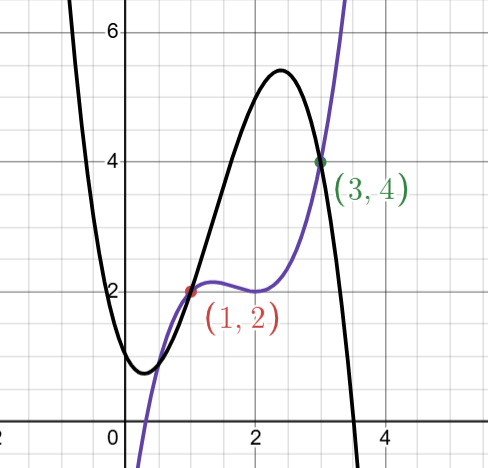
Note: Graphically, when two different polynomials evaluate to the same $y$-value for a given $x$, it means that they intersect at that point. For example:

$$ p(x) = x^2 \quad \text{and} \quad q(x) = 2x. $$

At $x=2$, both give $y=4$, so they intersect at the point $(2,4)$. In this case, we’re dealing with different polynomials. Another possibility for having the same $y$ for a given $x$ is that they are actually the same polynomial! In that case, they will have the same $y$ for all values of $x$, not just for some particular values of $x$.

In the case of $p(x)$ and $q(x)$, they are equal for at least n + 1 different values of $x$. This can be mathematically expressed as:

$$ p(x_i)=q(x_i) \space\space\forall i \in \{0,1,\dots, n\} $$

So, the difference between $p(x)$ and $q(x)$ at all $n+1$ points will be zero. That is,

$$ r(x_i) =p(x_i)- q(x_i) = 0 \space\space\forall i \in \{0,1,\dots, n\}$$

Therefore, $r(x)$ evaluates to zero at $n+1$ points, which implies that it is a zero polynomial. Let us see more clearly why.

A zero polynomial is one that evaluates to zero for all values of $x$. The simplest example of a zero polynomial is:

$$ p(x) = 0$$

Another way of looking at this is, if our domain of polynomial evaluation – the set of points at which the polynomial can be evaluated – is, say, $S=\{x_0, x_1 \cdots, x_{n-1}\}$, then a zero polynomial for this domain can be:

$$ p(x)=(x-x_0)(x-x_1)\cdots (x-x_{n-1})$$

Because,

$$ p(x) = 0 \quad \forall \quad x\in \{x_0,x_1,\cdots x_{n-1}\}$$

We could have many more zero polynomials for the domain $S$ such as:

$$ f_1(x)=p(x)\\f_2(x)=p(x)^2\\f_3(x)=0\cdot p(x)$$

Notice that each of $f_1(x), f_2(x)$ and $f_3(x)$ evaluates to zero for the domain $S$, and thus is a zero polynomial. We can have many more. The most primitive one being $f_3(x)=0$, i.e. the constant zero itself.

Note: If the domain $S$ is taken as the set of all real numbers, then the only zero polynomial we can have is $f(x)=0$, since no other polynomial will evaluate to zero for all real numbers.

Now observe the number of roots and degree for each of the example zero polynomials we looked at.

Roots of a polynomial are the values in the domain for which the polynomial evaluates to zero, whereas the degree of a polynomial is the highest power of the variable as you well know.

• $f_1(x):$ Roots- $n$, Degree- $n$
• $f_2(x):$ Roots- $n$, Degree- $2n$
• $f_3(x):$ Roots- $n$, Degree- $0$

All of them evaluate to zero on $S$; therefore, the number of roots is $n$, whereas the degree can be varied by modifying $p(x)$, whose degree is $n$.

Also note that $f_3(x)=0$ has the number of roots greater than its degree. This is only possible in the case of a zero polynomial, specifically the primitive one $f_3(x)=0$. Otherwise, the number of roots is always less than or equal to the degree.

Consider a non-zero polynomial of degree $n$; it can have at most $n$ roots (or intersections with the $x$-axis). The primitive zero polynomial is the only exception, as it has more roots than its degree.

For example, a quadratic equation of degree $2$, such as $q(x)=x^2-3x+2$, has two roots, i.e. $x=1$ and $x=2$.

For a quadratic equation to have more than two roots, it must be equal to zero, i.e. $q(x)=0$.

Now, coming back to our argument: since $r(x)$ evaluates to zero at $n+1$ points, it must have at least $n+1$ roots, which is greater than its degree $n$. Therefore $r(x)$ must be equal to zero.

$$ p(x)-q(x)=r(x)=0$$

This implies that $p(x)=q(x)$, meaning they are the same polynomial. Therefore, the polynomial of lowest degree that interpolates a set of $n+1$ distinct points is unique.