Visual representation of the roots of unity

The property that if $\omega$ is a $k$-th root of unity, then $\omega^i$ and $\omega^{i+k/2}$ are additive inverses may seem a little abstract — this chapter introduces a visual that makes this concept easier to remember.

Recall that the $k$-th roots of unity are generated by taking the primitive $k$-th root of unity $\omega$ and raising it to successive powers. For example, if $k=4$, we compute the 4-th roots of unity as

• $\omega^0=1$
• $\omega^1=\omega$
• $\omega^2=\omega^2$
• $\omega^3=\omega^3$

If we were to keep going, the exponents would wrap around modulo 4:

• $\omega^4=1$ (by definition of being a 4-th root of unity)
• $\omega^5=\omega^4\omega=1\cdot\omega =\omega$
• $\omega^6=\omega^4\omega^2=1\cdot\omega^2=\omega^2$
• $\omega^7=\omega^4\omega^3=1\cdot\omega^3=\omega^3$
• $\omega^8=\omega^4\omega^4=1$
• $\omega^9=\omega^4\omega^4\omega=\omega$

and so on.

Note that the exponent “wraps around” at each multiple of four. Thus, for any $\omega^i$ and $\omega^j$, $\omega^i\omega^j=\omega^{i+j\pmod k}$. Since $k=4$ in our example, we have that $\omega^i\omega^j=\omega^{i+j\pmod 4}$

Now recall that addition modulo $k$ can be represented as a “clock.” Here, our clock consists of the “hour markers” 0, 1, 2, 3, which are the exponents of $\omega$

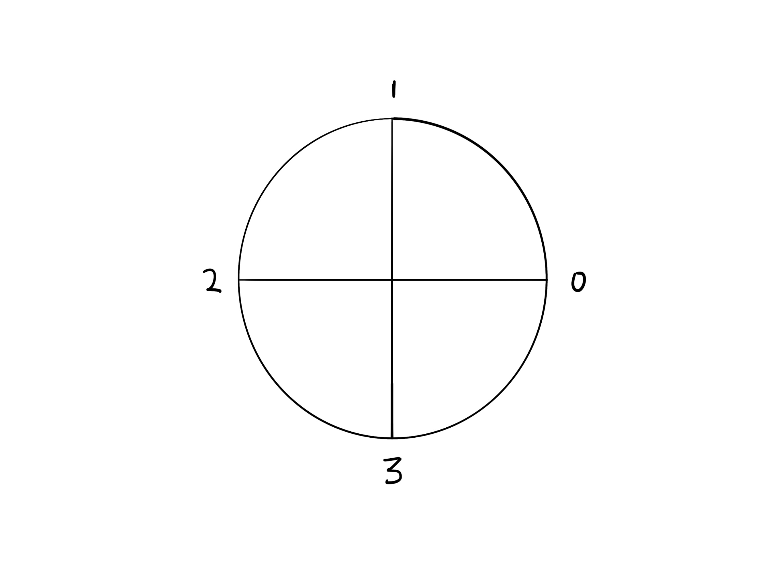
One way to think about this is

“adding two numbers $i$ and $j$ on the clock is equivalent to multiplying the roots of unity that have exponents $i$ and $j$ i.e. $\omega^i$ and $\omega^j$.”

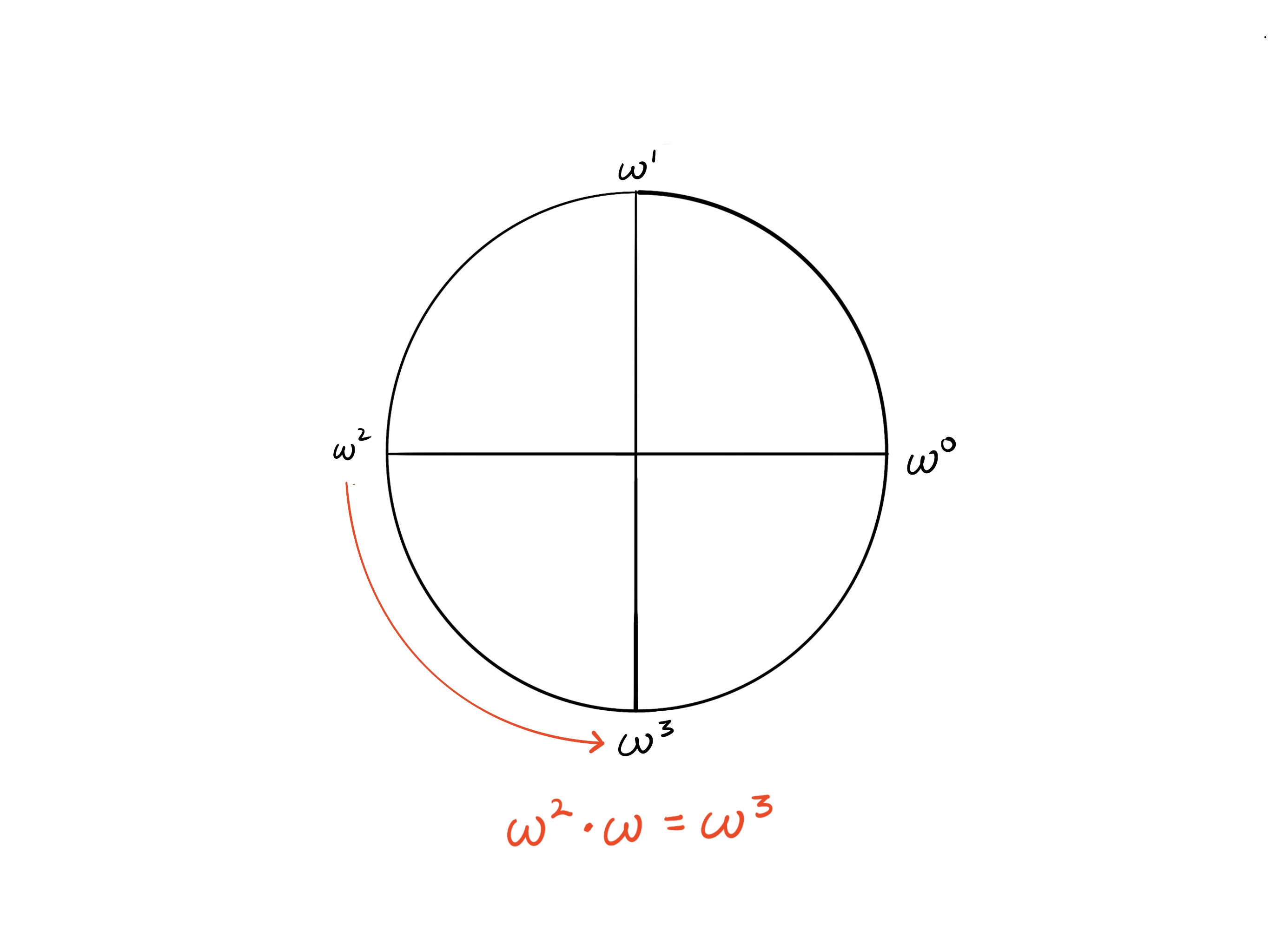
If we take any root of unity and add 1 to the exponent, this is equivalent to multiplying that root of unity by $\omega^1$ (or just $\omega$). For example, multiplying $\omega^2$ by $\omega$ is the same as adding one to the exponent to get $\omega^3$.

Therefore, multiplying a $k$-th root of unity by $\omega$ or adding 1 to the exponent is the same as taking $1/k$-th step around the circle.

For example, if we multiply $\omega^2$ by $\omega,$ we get $\omega^3$, which equals moving forward 1/4-th step:

We can think of generating the roots of unity by starting with $\omega^0$ and repeatedly adding 1 to the exponent to produce $\omega^1, \omega^2, \omega^3$, and so on until we reach $\omega^{k}$ at which point the results will wrap around modulo $k$. This is exactly the same as taking $k$ steps around the circle.

Visualizing congruences with the unit circle

Let’s expand this circle to include more congruences.

If we multiply $\omega^3$ and $\omega^2$, we will get $\omega^5$, which is congruent to $\omega$, exactly as the chart suggests:

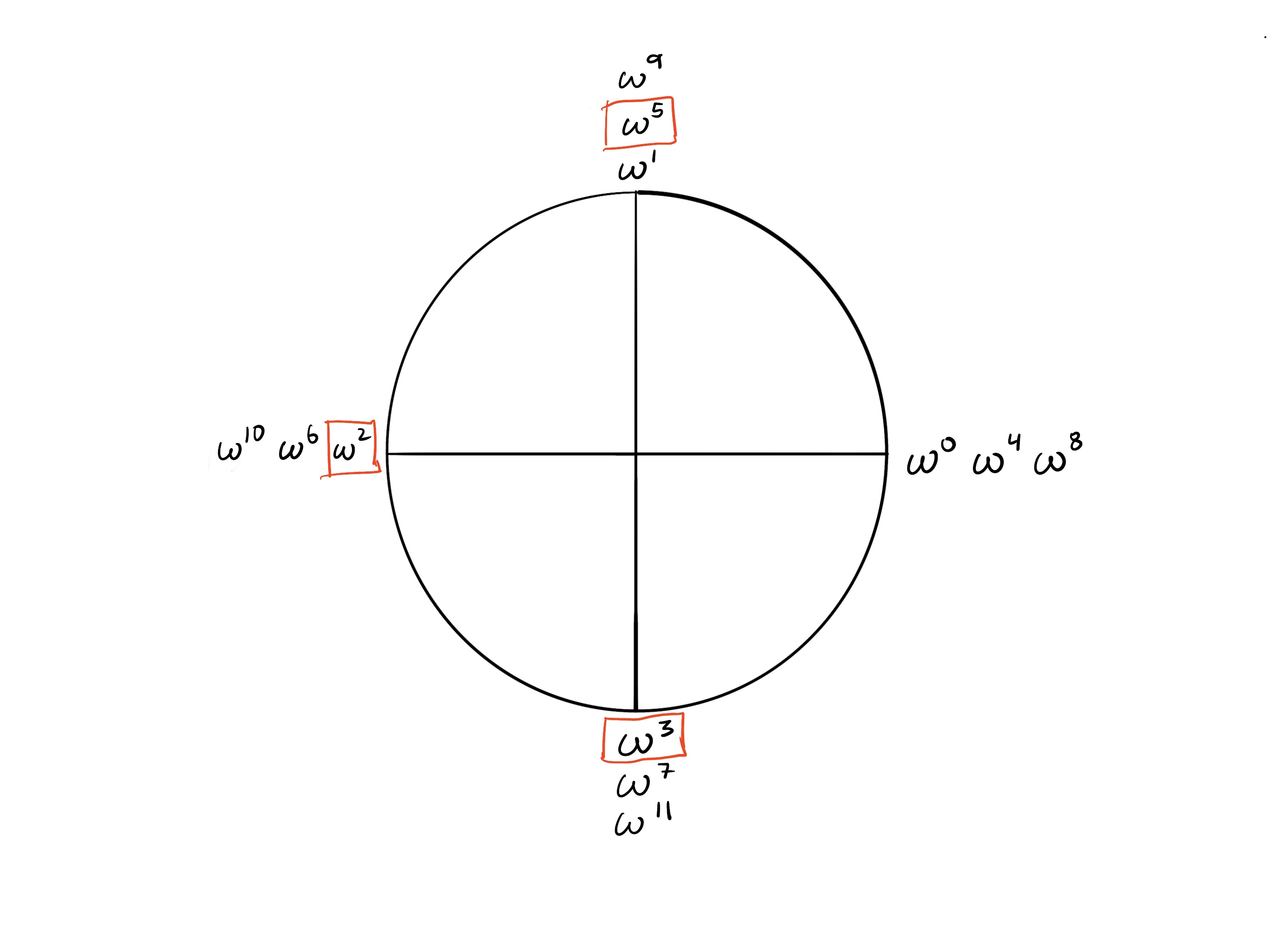
Another way to think about this is starting at $\omega^2$ and taking 3 steps forward:

Points k/2 steps apart

Since it takes $k$ steps to “walk around” the circle, $k/2$ steps takes you from a point to the opposite point.

Now observe in the circle of $k=4$ that opposite points are additive inverses of each other (they sum to zero). Recall that $-1\equiv\omega^{k/2}$. Since k = 4, $\omega^2 =-1.$

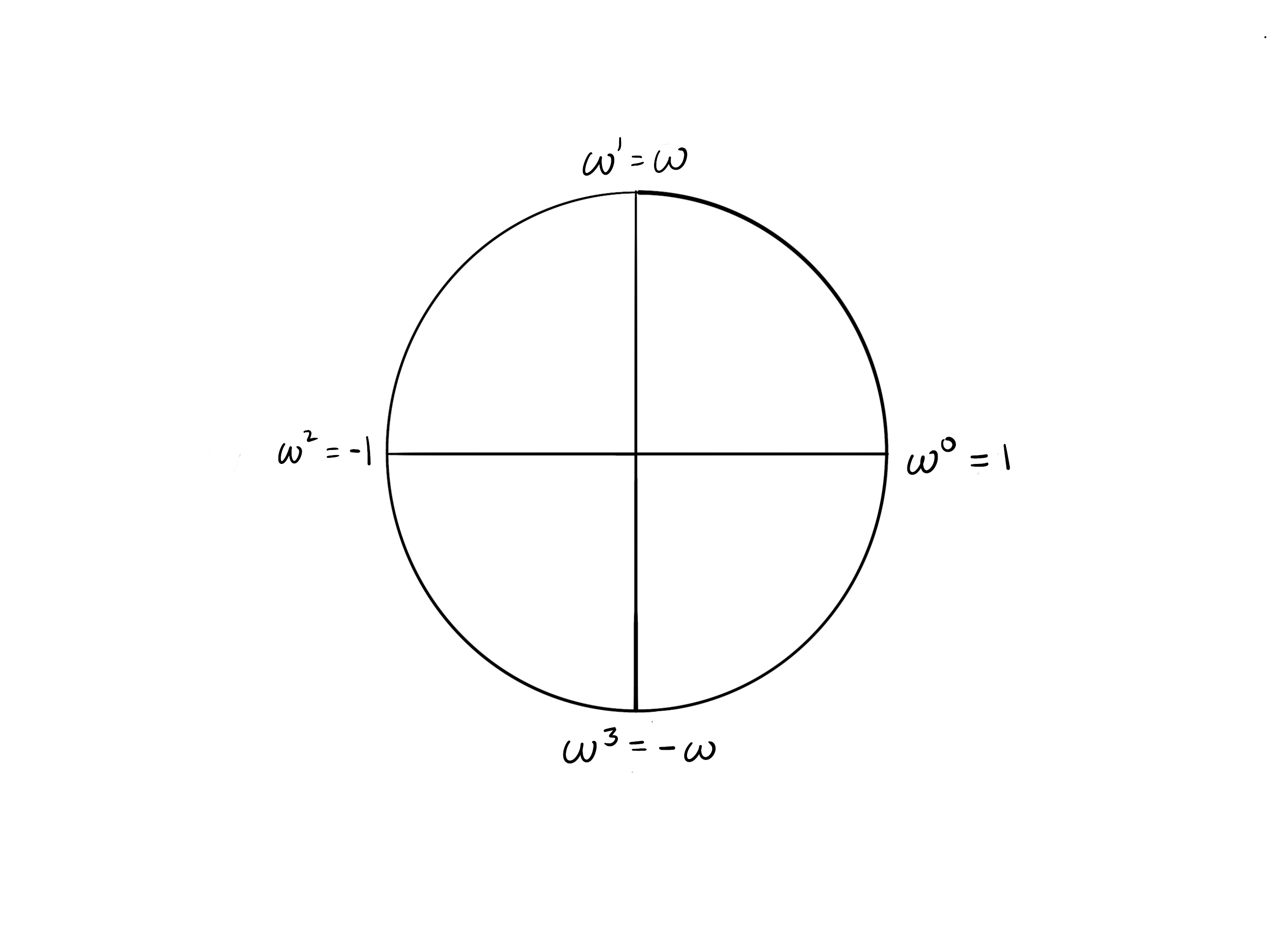
In the $k=4$ example, we have that

• $\omega^0+\omega^2\equiv1+(-1)=0$
• $\omega^1+\omega^3\equiv\omega+(-\omega)=0$

Note that we are now adding the roots of unity together, not multiplying them, so the addition of exponents rule does not apply! Don’t confuse $\omega^0+\omega^2$ with $\omega^0\cdot\omega^2$! Roots of unity are finite field elements, and fields have 2 operations: addition and multiplication.

Examples with other values of k

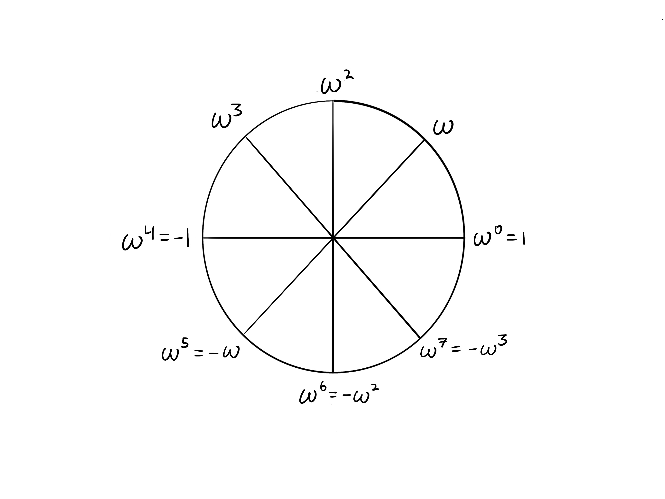
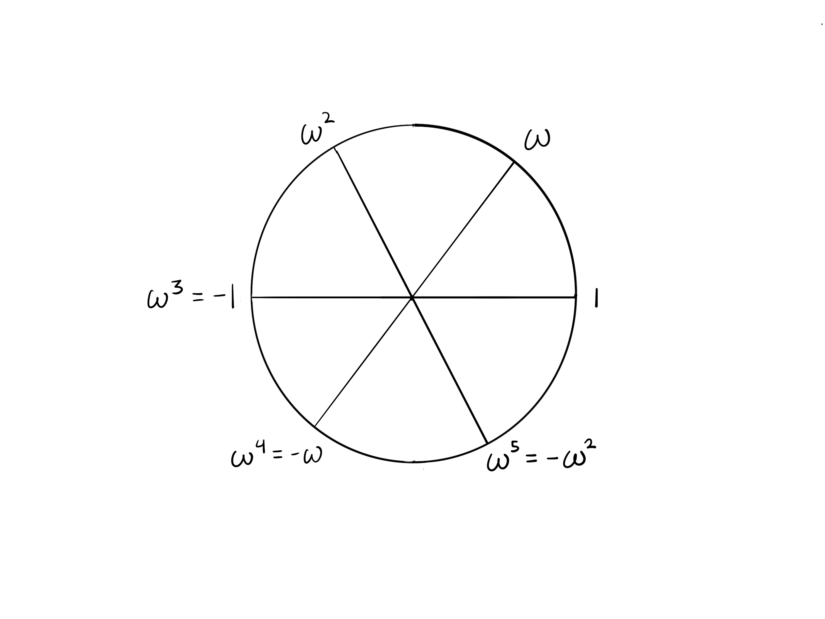
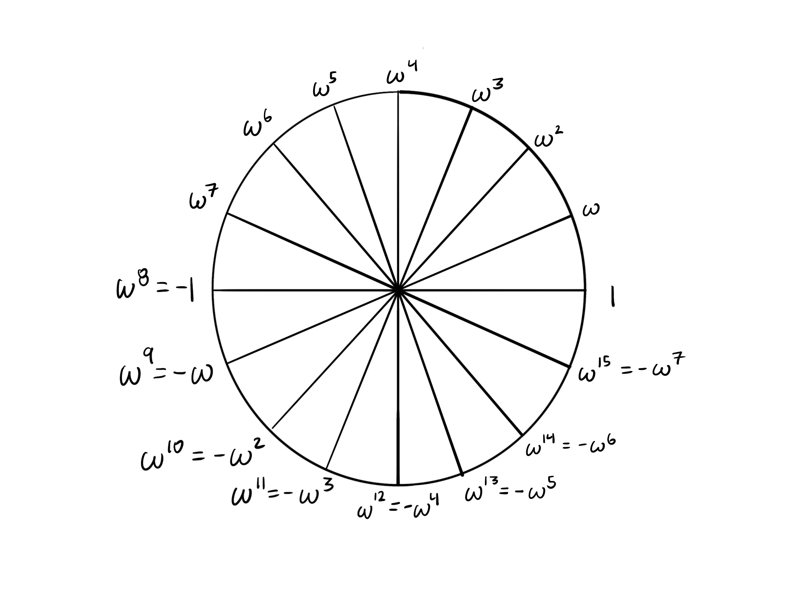
If the circle is partitioned into $k$ segments, then taking $k/2$ steps takes you to the opposite side. In each of the cases shown here, we see that opposite points are additive inverses.

k = 8

k = 6

k = 16

Summary

To remember that $\omega^i+\omega^{i+k/2}$ are additive inverses (their sum is zero), we draw a circle with $k$ points where each step is a multiplication by $\omega.$ The opposite points will be additive inverses.

The circle diagram will also be very useful for visualizing subgroups of the roots of unity as well as square roots — we will show those visualizations in the upcoming chapters.