The Schwartz-Zippel Lemma and its application to Zero Knowledge Proofs

Nearly all ZK-Proof algorithms rely on the Schwartz-Zippel Lemma to achieve succintness.

The Schwartz-Zippel Lemma states that if we are given two polynomials $p(x)$ and $q(x)$ with degree $d_p$ and $d_q$ respectively, and if $p(x) \neq q(x)$, then the number of points where $p(x)$ and $q(x)$ intersect is less than or equal to $\mathsf{max}(d_p, d_q)$.

Let’s consider a few examples.

Example polynomials and the Schwartz-Zippel Lemma

A straight line crossing a parabola

Consider the polynomial $p(x) = x$ and $q(x) = x^2$. They intersect at $x = 0$ and $x = 1$.

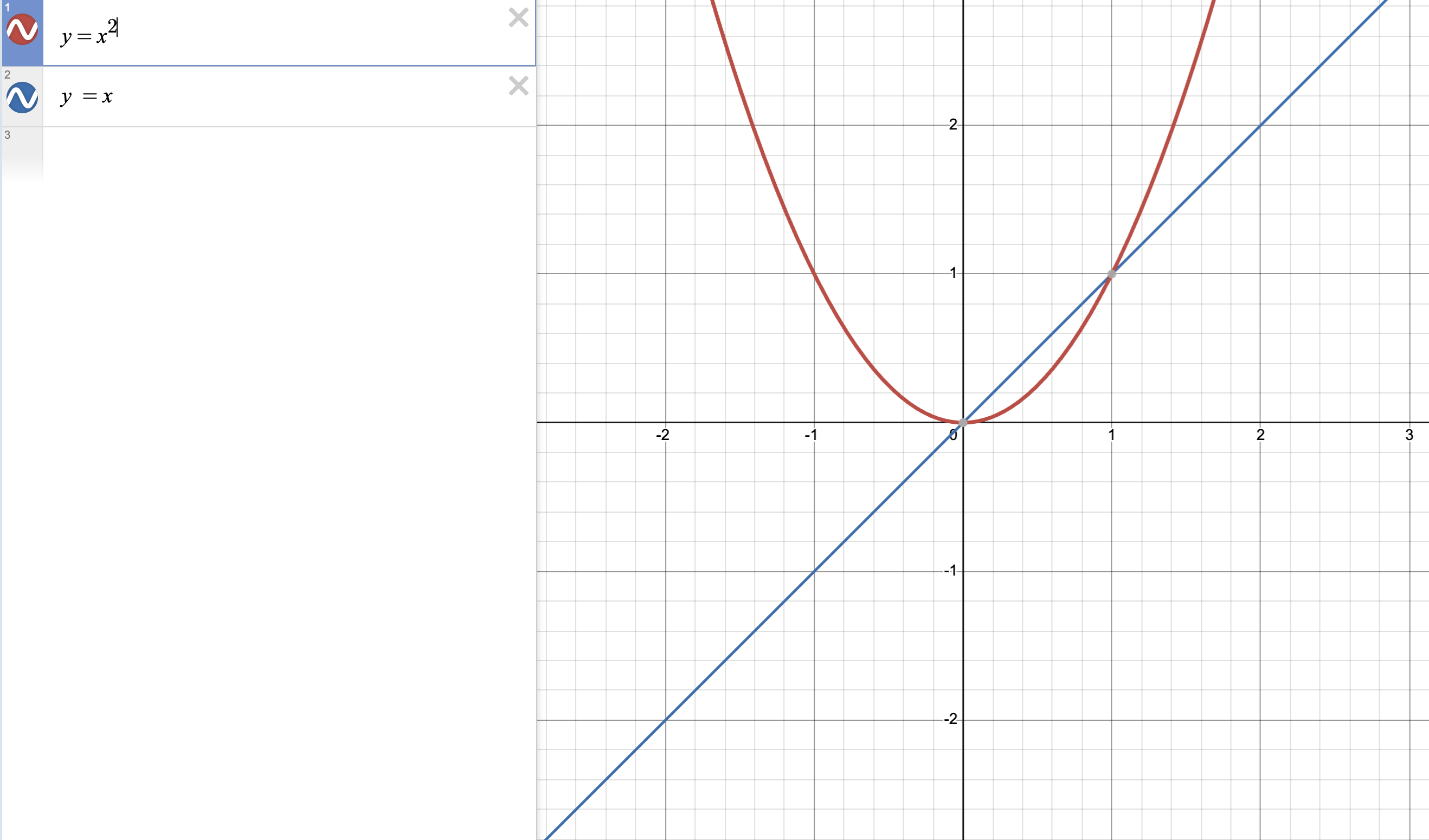
They intersect at two points, which is the maximum degree between the polynomials $y = x$ and $y = x^2$.

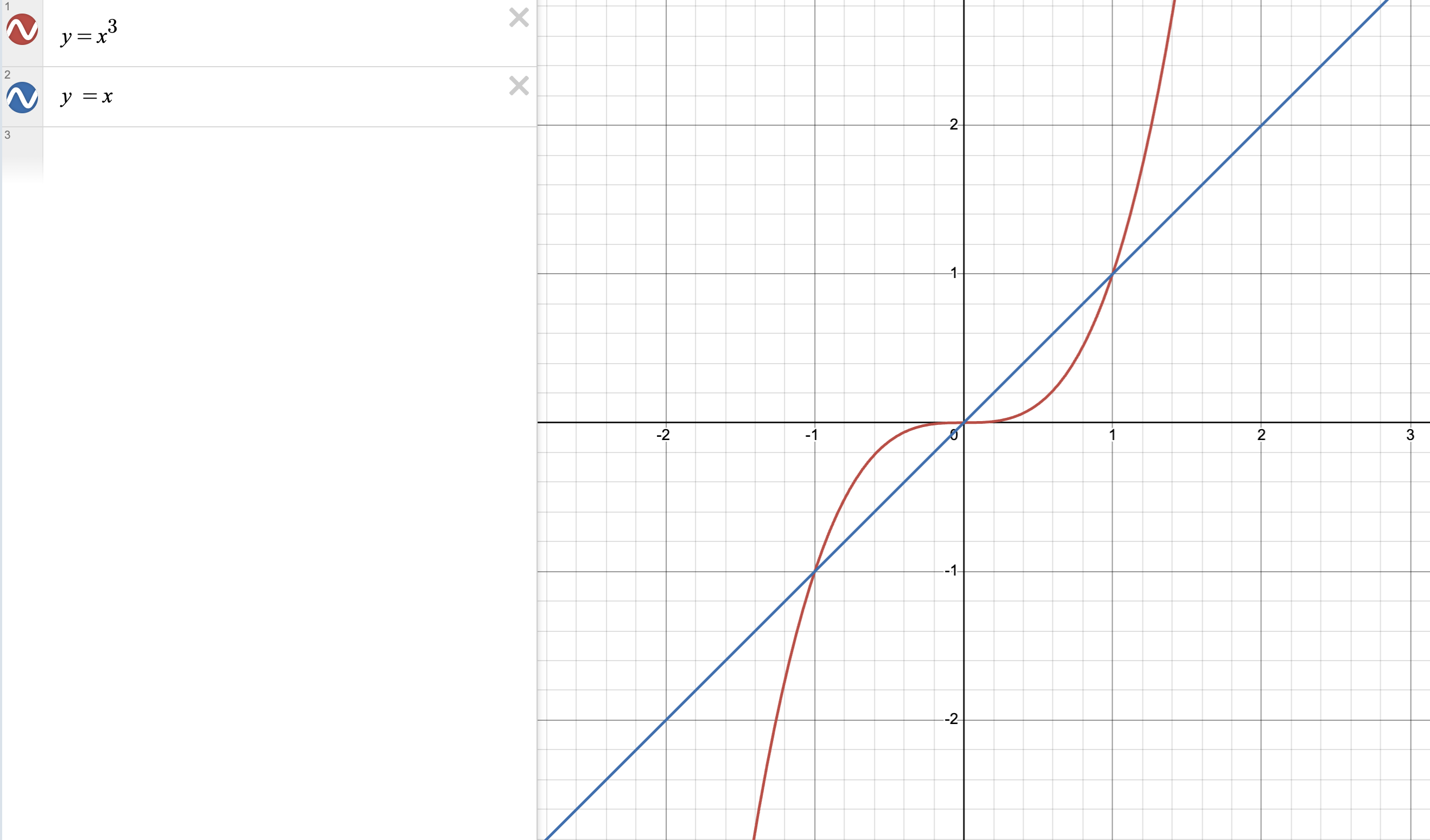
A degree three polynomial and a degree one polynomial

Consider the polynomials $p(x) = x^3$ and $q(x) = x$. The polynomials intersect at $x = -1$, $x = 0$, and $x = 1$ and nowhere else. The number of intersections is bounded by the maximum degree of the polynomials, which in this case is 3.

Polynomials in finite fields and the Schwartz-Zippel Lemma

The Schwartz-Zippel Lemma holds for polynomials in finite fields (i.e. all computations are done modulo a prime $p$).

Polynomial equality testing

We can test that two polynomials are equal by checking if all their coefficients are equal, but this takes $\mathcal{O}(d)$ time, where $d$ is the degree of the polynomial.

If instead we can evaluate the polynomials at a random point $u$ compare the evaluations in $\mathcal{O}(1)$ time.

That is, in a finite field $\mathbb{F}_{p}$, we pick a random value $u$ from $[0,p)$. Then we evaluate $y_f=f(u)$ and $y_g=g(u)$. If $y_f = y_g$, then one of two things must be true:

1. $f(x) = g(x)$
2. $f(x) \neq g(x)$ and we picked one of the $d$ points where they intersect where $d = \mathsf{max}(\deg(f), \deg(g))$

If $d << p$, then situation 2 is unlikely to the point of being negligible.

For example, if the field $\mathbb{F}_{p}$ has $p \approx 2^{254}$ (a little smaller than a uint256), and if the polynomials are not more than one million degree large, then the probability of picking a point where they intersect is

$$ \frac{1\times 10^6}{2^{254}} \approx \frac{2^{20}}{2^{254}} \approx \frac{1}{2^{234}} \approx \frac{1}{10^{70}} $$

To put a sense of scale on that, the number of atoms in the universe is about $10^{78}$ to $10^{82}$, so it is extremely unlikely that we will pick a point where the polynomials intersect, if the polynomials are not equal.

Using the Schwartz-Zippel Lemma to test if two vectors are equal

We can combine Lagrange interpolation with the Schwartz-Zippel Lemma to test if two vectors are equal.

Normally, we would test vector equality by comparing if each of the $n$ components of the vectors are equal.

Instead, if we use a common set of $x$ values (say $[1,2,..,n]$) to interpolate the vectors:

1. we can interpolate a polynomial for each vector $f(x)$ and $g(x)$
2. pick a random point $u$
3. evaluate the polynomials at $u$
4. check if $f(u) = g(u)$

Although computing the polynomials is more work, the final check is much cheaper.

Here is an example of carrying out this computation in Python:

import galois
import numpy as np

p = 103
GF = galois.GF(p)

xs = GF(np.array([1,2,3]))

# arbitrary vectors
v1 =  GF(np.array([4,8,19]))
v2 =  GF(np.array([4,8,19]))


def L(v):
    return galois.lagrange_poly(xs, v)

p1 = L(v1)
p2 = L(v2)

import random
u = random.randint(0, p)

lhs = p1(u)
rhs = p2(u)

# only one check required
assert lhs == rhs

Using the Schwartz-Zippel Lemma in ZK Proofs

Our end goal is for the prover to send a small string of data to the verifier that the verifier can quickly check.

Most of the time, a ZK proof is essentially a polynomial evaluated at a random point.

The difficulty we have to solve is that we don’t know if the polynomial is evaluated honestly — somehow we have to trust the prover isn’t lying when they evaluate $f(u)$.

But before we get to that, we need to learn how to represent and entire arithmetic circuit as a small set of polynomials evaluated at a random point, which is the motivation for Quadratic Arithmetic Programs.