Zero Knowledge Multiplication

Zero Knowledge Multiplication of Polynomials

Using the polynomial commitment scheme from the previous chapter, a prover can show that they have three polynomials $l(x)$, $r(x)$, and $t(x)$ and prove that $t(x) = l(x)r(x)$.

For this algorithm to work, the verifier must believe that the polynomial evaluations are correct — but this is something we showed in the previous chapter. Most of the steps here are simply repeating the polynomial commitment algorithm we did previously.

At a high level, the prover commits to $l(x)$, $r(x)$, and $t(x)$ and sends the commitments to the verifier. Then, the verifier chooses a random value for $x$ as $u$ and asks the prover to evaluate the polynomials at $u$. The verifier then checks that the evaluations were done correctly and that the evaluation for $l(x)$ multiplied by the evaluation for $r(x)$ equals the evaluation for $t(x)$.

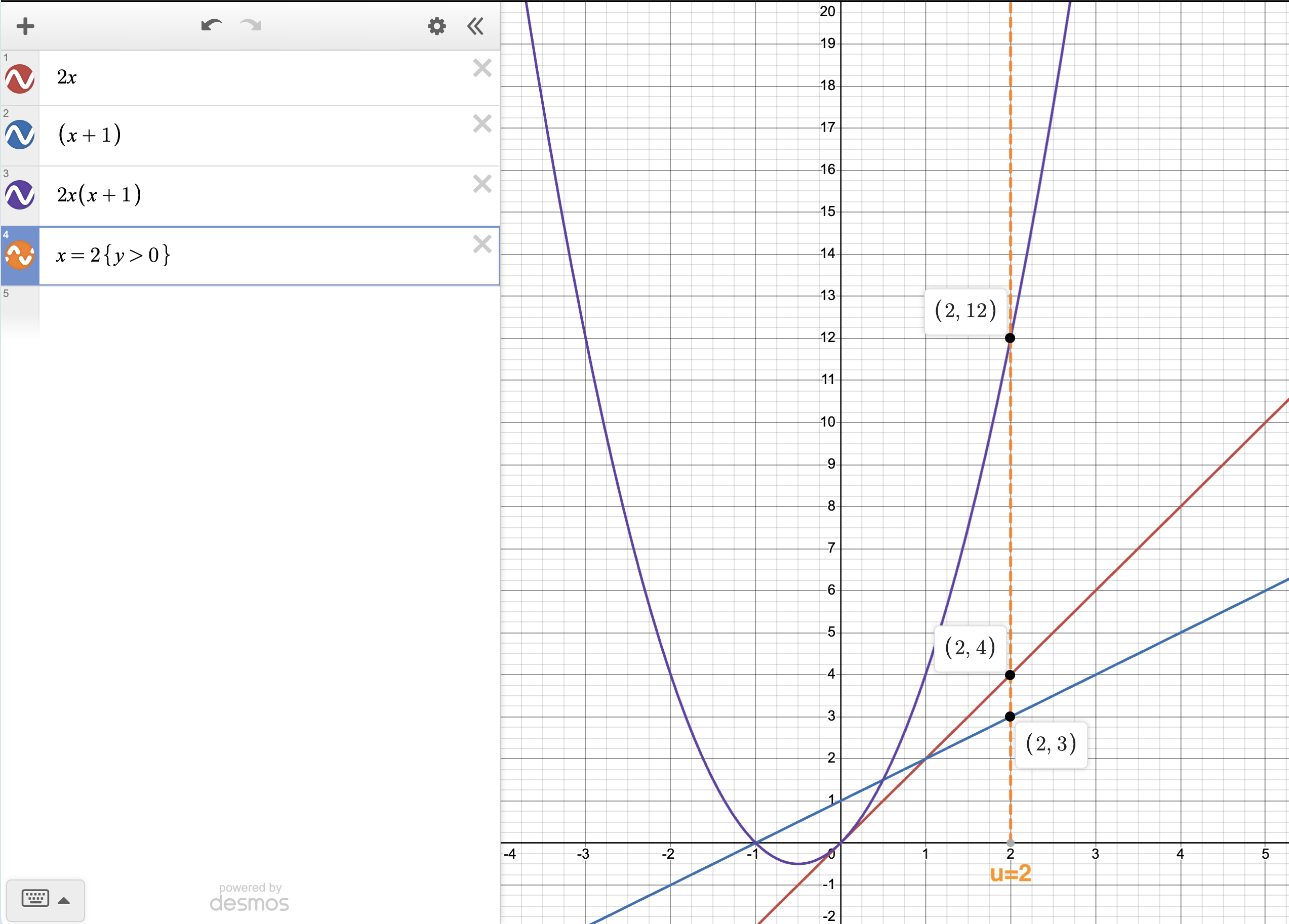
For example, suppose that the first polynomial is $l(x)=2x$ and the second is $r(x) = x + 1$. Then $t(x)=2x(x+1) = 2x^2+2$. The verifier can sample any random $x$ value, and the result of the product $l(x)r(x)$ will be $t(x)$. The plot below shows an example of the verifier choosing $x=2$:

The verifier would then check that $3 \times 4 = 12$ and accept the prover’s claim.

The Schwartz-Zippel lemma states that if $f(x) \neq g(x)$ then the probability that $f(u) = g(u)$ for some random value $u$ is less than $d/p$ where $d$ is the maximum degree of the two polynomials and $p$ is the order of the finite field. If $d \ll p$ ($d$ much much less than $p$), then the probability of $u$ being an intersection point of two non-equal polynomials is negligible.

Specifically, suppose the prover is lying and $l(x)r(x) \neq t(x)$. In that case, for a random $u$, $l(u)r(u) \neq t(u)$ with extremely high probability. If $l(x)r(x) \neq t(x)$, then $l(x)r(x)$ and $t(x)$ only intersect in at most $d$ points (the maximum degree of either $l(x)r(x)$ or $t(x)$), and it is extremely unlikely that the verifier would randomly pick a $u$ that is one of the $d$ intersection points.

To get a sense of scale, $d$ in our case is 2, but the curve order of our elliptic curves (and hence the order of the field) is about $2^{254}$. So if $t(x) \neq l(x)r(x)$, then the probability of $t(u) = l(u)r(u)$ is $1/2^{253}$ which is vanishingly small.

We now describe the algorithm in detail, and then show an optimization.

Steps to prove knowledge of polynomial multiplication

The prover commits two linear (degree 1) polynomials $l(x)$, $r(x)$, a quadratic (degree 2) polynomial $t(x)$, and sends the commitments to the verifier. The verifier responds with a random value $u$, and the prover evaluates $l_u = l(u)$, $r_u = r(u)$, and $t_u = t(u)$ along with the proofs of evaluation $\pi_l, \pi_r, \pi_t$. The verifier asserts that all the polynomials were evaluated properly and that $t_u = l_ur_u$.

Setup

The prover and verifier agree on elliptic curve points $G$ and $B$ with an unknown discrete log relationship (i.e. the points are chosen randomly).

Prover commits to $l(x)$, $r(x)$, and $t(x)$

The prover creates three polynomials:

$$ \begin{align*} l(x) &= a + s_Lx \\ r(x) &= b + s_Rx \\ t(x) &= l(x)r(x) = (a + s_Lx)(b + s_Rx) = ab+(as_R+bs_L)x+s_Ls_Rx^2\\ \end{align*} $$

So they need to produce a total of 7 Pedersen commitments for each of the coefficients, which will require seven blinding terms $\alpha_0, \alpha_1, \beta_0, \beta_1, \tau_0, \tau_1, \tau_2$

$$ \begin{align*} L_0&=aG + \alpha_0B &&\text{// constant coefficient of }l(x)\\ L_1&=s_LG + \alpha_1B &&\text{// linear coefficient of }l(x)\\ \\ R_0&=bG + \beta_0B &&\text{// constant coefficient of }r(x)\\ R_1&=s_RG + \beta_1B &&\text{// linear coefficient of }r(x)\\ \\ T_0 &= abG + \tau_0 B &&\text{// constant coefficient of }t(x)\\ T_1 &=(as_R + bs_L)G + \tau_1B &&\text{// linear coefficient of }t(x)\\ T_2 &= s_Ls_RG + \tau_2B &&\text{// quadratic coefficient of }t(x) \end{align*} $$

The prover sends $(L_0, L_1, R_0, R_1, T_0, T_1, T_2)$ to the verifier.

Verifier generates random scalar $u$

… and sends the field element $u$ to the prover.

Prover evaluates the three polynomials and creates three proofs

The prover plugs in $u$ to the polynomials and computes the sum of the blinding terms of the polynomial coefficient commitments when $u$ is applied.

$$ \begin{align*} l_u &= a + s_Lu\\ r_u &= b + s_Ru\\ t_u &= ab + (as_R + bs_l)u + s_Ls_Ru^2\\ \\ \pi_l &= \alpha_0 + \alpha_1u \\ \pi_r &= \beta_0 + \beta_1u \\ \pi_t &= \tau_0 + \tau_1u + \tau_2u^2 \end{align*} $$

The prover sends the values $(l_u, r_u, t_u, \pi_l, \pi_r, \pi_t)$ to the verifier. Note that these are all field elements, not elliptic curve points.

Final verification step

The verifier checks that each of the polynomials were evaluated correctly and that the evaluation of $t(u)$ is the product of the evaluation of $l(u)$ and $r(u)$. The first three checks are proofs that the polynomial was evaluated correctly with respect to the commitment to the coefficients, and the last check verifies that the output of the polynomials have the product relationship as claimed.

$$ \begin{align*} l_uG + \pi_l B &\stackrel{?}= L_0+L_1u &&\text{// Check that }l(u) \text{ was evaluated correctly}\\ r_uG + \pi_r B &\stackrel{?}= R_0+R_1u &&\text{// Check that }r(u) \text{ was evaluated correctly}\\ t_uG + \pi_t B &\stackrel{?}= T_0+T_1u+T_2u^2&&\text{// Check that }t(u) \text{ was evaluated correctly}\\ t_u &\stackrel{?}= l_ur_u &&\text{// Check that }t(u)=l(u)r(u) \end{align*} $$

When we expand the terms, we see they balance if the prover was honest: $$ \begin{align*} \underbrace{(a + s_Lu)}_{l_u}G + \underbrace{(\alpha_0 + \alpha_1u)}_{\pi_l} B &\stackrel{?}= \underbrace{(aG + \alpha_0B)}_{L_0}+\underbrace{(s_LG + \alpha_1B)}_{L_1}u \\ \underbrace{(b + s_Ru)}_{r_u}G + \underbrace{(\beta_0 + \beta_1u)}_{\pi_r} B &\stackrel{?}= \underbrace{(bG + \beta_0B)}_{R_0}+\underbrace{(s_RG + \beta_1B)}_{R_1}u \\ \underbrace{(ab + (as_R + bs_l)u + s_Ls_Ru^2)}_{t_u}G + \underbrace{(\tau_0 + \tau_1u + \tau_2u^2)}_{\pi_t} B &\stackrel{?}= \underbrace{(abG + \tau_0 B)}_{T_0}+\underbrace{(as_R + bs_L+ \tau_1B)}_{T_1}u+\underbrace{(s_Ls_R+ \tau_2B)}_{T_2}u^2 \\ t_u &\stackrel{?}= l_ur_u \end{align*} $$

Optimization: sending fewer commitments

In the first step, the prover sends 7 elliptic curve points, and in the final step, the verifier checks 4 equalities. We can improve the algorithm to only send 5 elliptic curve points and do 3 equality checks.

This is done by putting the constant coefficients of $l(x)$ and $r(x)$ into a single commitment and the linear coefficients of those polynomials into a separate commitment. By way of reminder, we defined $l(x)$ and $r(x)$ as

$$\begin{align*} l(x) &= a + s_Lx \\ r(x) &= b + s_Rx \\ \end{align*}$$

so $a$ and $b$ are the constant coefficients, and $s_L$ and $s_R$ are the linear coefficients.

This is similar to how we would commit a vector. We are in a sense committing the constant coefficients as a vector and the linear coefficients as another vector.

Setup

During the setup, we now need 3 elliptic curve points: $G$, $H$, and $B$.

Polynomial commitment

$$ \begin{align*} A &= aG + bH + \alpha B &&\text{// commit the constant terms}\\ S &= s_LG + s_RH + \beta B &&\text{// commit the linear terms}\\ T_0 &= abG + \tau_0 B &&\text{// commit the constant coefficient of } t(x) \\ T_1 &=(as_R + bs_L)G + \tau_1B &&\text{// linear coefficient of }t(x)\\ T_2 &= s_Ls_RG + \tau_2B &&\text{// quadratic coefficient of }t(x) \end{align*} $$

Note that the coefficients of $l(x)$ are applied to $G$ and the coefficients of $r(x)$ are applied to $H$. The prover sends $(A, S, T_0, T_1, T_2)$ to the verifier, who responds with $u$.

Polynomial evaluation

$$ \begin{align*} l_u &= l(u) = a + s_Lu\\ r_u &= r(u) = b + s_Ru\\ t_u &= t(u) = l(u)r(u) = ab + (as_R + bs_L)u + s_Ls_Ru^2\\ \pi_{lr} &= \alpha + \beta u \\ \pi_t &= \tau_0 + \tau_1u + \tau_2u^2 \end{align*} $$

$l_u$, $r_u$, $t_u$, $\pi_{lr}$, and $\pi_t$ are computed as before, but the proof of evaluations for $l(x)$ and $r(x)$, which were formerly $\pi_l$ and $\pi_r$ are combined into a single one: $\pi_{lr}$.

Final verification

$$ \begin{align*} A + Su &\stackrel{?}= l_uG + r_uH+\pi_{lr}B \\ t_uG + \pi_tB &\stackrel{?}= T_0 + T_1u + T_2u^2 \\ t_u &\stackrel{?}= l_ur_u \end{align*} $$

The check $A + Su \stackrel{?}= l_uG + r_uH+\pi_{lr}B$ expands to

$$ \underbrace{(aG + bH + \alpha B)}_A + \underbrace{(s_LG + s_RH + \beta B)u}_{Su} = \underbrace{(a + s_Lu)}_{l_u}G + \underbrace{(b + s_Ru)}_{r_u}H + \underbrace{(\alpha + \beta u)}_{\pi_{lr}}B $$

With some rearranging on the left-hand-side, we can see the equality check simultaneously checks that both $l(x)$ and $r(x)$ were evaluated correctly.

$$ (a + s_Lu)G + (b + s_Ru)H + (\alpha + \beta u)B=\underbrace{(a + s_Lu)}_{l_u}G + \underbrace{(b + s_Ru)}_{r_u}H + \underbrace{(\alpha + \beta u)}_{\pi_{lr}}B $$

As another way of looking at the check $A + Su \stackrel{?}= l_uG + r_uH+\pi_{lr}B$, consider the following visualization:

$$ \begin{align*} A &= &aG& + &bH &+ &\alpha B\\ Su &= &s_LuG& + &s_RuH &+ &\beta u B\\ &&\vcenter{\hbox{|}} \vcenter{\hbox{|}}&&\vcenter{\hbox{|}} \vcenter{\hbox{|}}&&\vcenter{\hbox{|}} \vcenter{\hbox{|}}\\ &&l(u)G&&r(u)H&&\pi_{lr}B \end{align*} $$

Zero Knowledge Multiplication of Scalars

Our proof that we multiplied two polynomials together correctly to obtain a third can be used to prove that we multiplied two scalars together to obtain a third. No changes to the algorithm are necessary, only a minor change in semantics (how we interpret the commitments).

Let’s say we want to prove that we carried out the multiplication $ab = v$.

Problem statement

$A$ is a commitment to $a$ and $b$, and $V$ is a commitment to $v$ where $v = ab$. We wish to prove that $A$ and $V$ are committed as claimed without revealing $a$, $b$, or $v$.

Solution

The high level idea is that a scalar can be turned into a polynomial by adding an arbitrarily chosen linear term, e.g. $a$ becomes $a + s_Lx$ and $b$ becomes $b + s_Rx$. $s_L$ and $s_R$ are chosen randomly by the prover.

When the polynomials $a + s_Lx$ and $b + s_Rx$ are multiplied together, the multiplication of $ab$ happens “inside” the polynomial multiplication.

$$(a + s_Lx)(b + s_Rx) = \boxed{ab} + (as_R + bs_L)x + s_Ls_rx^2$$

Recall the prover begins the algorithm by sending commitments:

$$ \begin{align*} A &= aG + bH + \alpha B &&\text{// commitment to }a\text{ and }b\\ S &= s_LG + s_RH + \beta B &&\text{// commit the linear terms}\\ V &= abG + \tau_0 B &&\text{// commit the product V} \\ T_1 &=(as_R + bS_L)G + \tau_1B &&\text{// linear coefficient of }t(x)\\ T_2 &= s_Ls_RG + \tau_2B &&\text{// quadratic coefficient of }t(x) \end{align*} $$

We simply change the “interpretation” of $A$ from being the constant terms of the polynomials to the constants $a$ and $b$ that we are multiplying. We change $T_0$ to $V$ to reflect the change of interpretation as a commitment to $V$ in the multiplication we are trying to prove we did correctly, i.e. $v = ab$.

Exercise: Fill in the missing Python code to implement the algorithm described above.

from py_ecc.bn128 import G1, multiply, add, FQ, eq
from py_ecc.bn128 import curve_order as p
import random

def random_element():
    return random.randint(0, p)

# these EC points have unknown discrete logs:
G = (FQ(6286155310766333871795042970372566906087502116590250812133967451320632869759), FQ(2167390362195738854837661032213065766665495464946848931705307210578191331138))

H = (FQ(13728162449721098615672844430261112538072166300311022796820929618959450231493), FQ(12153831869428634344429877091952509453770659237731690203490954547715195222919))

B = (FQ(12848606535045587128788889317230751518392478691112375569775390095112330602489), FQ(18818936887558347291494629972517132071247847502517774285883500818572856935411))

# utility function
def addd(A, B, C):
    return add(A, add(B, C))

# scalar multiplication example: multiply(G, 42)
# EC addition example: add(multiply(G, 42), multiply(G, 100))

# remember to do all arithmetic modulo p
def commit(a, sL, b, sR, alpha, beta, gamma, tau_1, tau_2):
    pass
    # return (A, S, V, T1, T2)


def evaluate(f_0, f_1, f_2, u):
    return (f_0 + f_1 * u + f_2 * u**2) % p

def prove(blinding_0, blinding_1, blinding_2, u):
    # fill this in
    # return pi
    pass

## step 0: Prover and verifier agree on G and B

## step 1: Prover creates the commitments
a = ...
b = ...
sL = ...
sR = ...
t1 = ...
t2 = ...

### blinding terms
alpha = ...
beta = ...
gamma = ...
tau_1 = ...
tau_2 = ...

A, S, V, T1, T2 = commit(a, sL, b, sR, alpha, beta, gamma, tau_1, tau_2)

## step 2: Verifier picks u
u = ...

## step 3: Prover evaluates l(u), r(u), t(u) and creates evaluation proofs
l_u = evaluate(a, sL, 0, u)
r_u = evaluate(b, sR, 0, u)
t_u = evaluate(a*b, t1, t2, u)

pi_lr = prove(alpha, beta, 0, u)
pi_t = prove(gamma, tau_1, tau_2, u)

## step 4: Verifier accepts or rejects
assert t_u == (l_u * r_u) % p, "tu != lu*ru"
assert eq(add(A, multiply(S, u)), addd(multiply(G, l_u), multiply(H, r_u), multiply(B, pi_lr))), "l_u or r_u not evaluated correctly"
assert eq(add(multiply(G, t_u), multiply(B, pi_t)), addd(V, multiply(T1, u), multiply(T2, u**2 % p))), "t_u not evaluated correctly"

Learn more

This article is part of a series on Bulletproof ZKPs.